Online Course top-rated
Credit Risk Modeling in Python

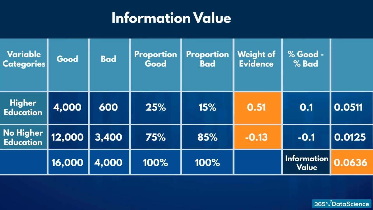
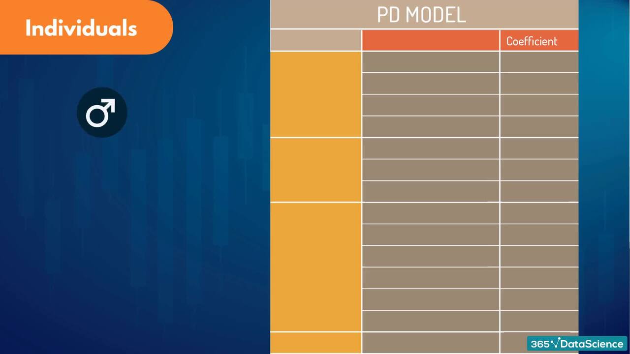
Blend credit risk modeling skills with Python programming: Learn how to estimate a bank’s loan portfolio's expected loss

4.8

862 reviews on
10,507 students already enrolled
  • Institute of Analytics
  • The Association of Data Scientists
  • E-Learning Quality Network
  • European Agency for Higher Education and Accreditation
  • Global Association of Online Trainers and Examiners

Skill level:

Advanced

Duration:

8 hours
  • Lessons (7 hours)
  • Practice exams (1.75 hours)

CPE credits:

12
CPE stands for Continuing Professional Education and represents the mandatory credits a wide range of professionals must earn to maintain their licenses and stay current with regulations and best practices. One CPE credit typically equals 50 minutes of learning. For more details, visit NASBA's official website: www.nasbaregistry.org

Accredited

certificate

What you learn

  • Master retail banking value drivers and credit risk modeling fundamentals.
  • Understand credit risk modeling concepts like PD, LGD, EAD, and Basel II.
  • Apply logistic regression in Python for accurate credit risk prediction.
  • Boost your data cleaning and processing skills with real-world loan data.
  • Acquire specialized credit risk modeling skills to enhance your resume.
  • Become invaluable for data scientist roles in the retail banking sector.

Topics & tools

TheoryPythonData AnalysisProgrammingCredit RiskLogistic RegressionData PreprocessingFinance SkillsIndustry Specialization

Your instructor

Course OVERVIEW

Description

CPE Credits: 12 Field of Study: Information Technology
Delivery Method: QAS Self Study
Credit risk modeling is the place where data science and fintech meet. It is one of the most important activities conducted in a bank, with the most attention since the recession. At present, it is the only comprehensive credit risk modeling course in Python available online – taking you from preprocessing, through probability of default (PD), loss given default (LGD) and exposure at default (EAD) modeling, all the way to calculating expected loss (EL).

Prerequisites

  • Python (version 3.8 or later), pandas library, and a code editor or IDE (e.g., Jupyter Notebook, Spyder, or VS Code)
  • Basic familiarity with Python programming is required.
  • Familiarity with NumPy is helpful but not mandatory.

Advanced preparation

Curriculum

68 lessons 80 exercises 5 exams
  • 1. Introduction
    38 min
    We start by explaining why credit risk is important for financial institutions. We also define ground 0 terms, such as expected loss, probability of default, loss given default and exposure at default.
    38 min
    We start by explaining why credit risk is important for financial institutions. We also define ground 0 terms, such as expected loss, probability of default, loss given default and exposure at default.
    What does the course cover Free
    What is credit risk and why is it important? Free
    Exercise Free
    Expected loss (EL) and its components: PD, LGD and EAD Free
    Exercise Free
    Capital adequacy, regulations, and the Basel II accord Free
    Exercise Free
    Basel II approaches: SA, F-IRB, and A-IRB Free
    Exercise Free
    Different facility types (asset classes) and credit risk modeling approaches Free
    Exercise Free
  • 2. Setting up the environment
    2 min
    Here you will learn how to set up Python 3 and load up Jupyter. We’ll also show you what the Anaconda Prompt is and how you can use it to download and import new modules.
    2 min
    Here you will learn how to set up Python 3 and load up Jupyter. We’ll also show you what the Anaconda Prompt is and how you can use it to download and import new modules.
    Setting up the environment Free
    Installing the relevant packages Free
  • 3. Dataset description
    9 min
    Our example focuses on consumer loans. Since there are more than 100 potential features, we've devoted a complete section to explain why some features are chosen over others.
    9 min
    Our example focuses on consumer loans. Since there are more than 100 potential features, we've devoted a complete section to explain why some features are chosen over others.
    Our example: consumer loans. A first look at the dataset Free
    Exercise Free
    Dependent variables and independent variables Free
    Exercise Free
  • 4. General preprocessing
    29 min
    Each raw datasets has its drawbacks. While most preprocessing is model specific, in some cases (like missing values imputation), we could generalize the data preparation.
    29 min
    Each raw datasets has its drawbacks. While most preprocessing is model specific, in some cases (like missing values imputation), we could generalize the data preparation.
    Importing the data into Python Free
    Exercise Free
    Preprocessing few continuous variables Free
    Preprocessing few continuous variables Homework Free
    Exercise Free
    Preprocessing few discrete variables Free
    Exercise Free
    Check for missing values and clean Free
    Check for missing values and clean Homework Free
    Exercise Free
  • 5. PD model: data preparation
    117 min
    Once we have completed all general preprocessing, we dive into model-specific preprocessing. We employ fine classing, coarse classing, weight of evidence and information value criterion to achieve the probability of default preprocessing. Conventionally, we should turn all variables into dummy indicators prior to modeling.
    How is the PD model going to look like?
    Exercise
    Dependent variable: Good/ Bad (default) definition
    Exercise
    Constructing independent variables
    Exercise
    Information value
    Exercise
    Data preparation. Splitting data
    Exercise
    Data preparation. Preprocessing one discrete variable
    Exercise
    Data preparation. Preprocessing discrete variables: automating calculations
    Exercise
    Data preparation. Preprocessing discrete variables: visualizing results
    Data Preparation. Preprocessing Discrete Variables: Creating Dummies (part 1)
    Exercise
    Data Preparation. Preprocessing Discrete Variables: Creating Dummies (part 2)
    Data Preparation. Preprocessing Discrete Variables: Creating Dummies (part 2)
    Exercise
    Data preparation. Preprocessing continuous variables: automating calculations
    Exercise
    Data preparation. Preprocessing continuous variables: creating dummies (part 1)
    Exercise
    Data preparation. Preprocessing continuous variables: creating dummies (part 2)
    Data preparation. Preprocessing continuous variables: creating dummies (part 2)
    Exercise
    Data preparation. Preprocessing continuous variables: creating dummies (part 3)
    Creating dummies Homework
    Exercise
    Data preparation. Preprocessing the test dataset
    Practice exam
  • 6. PD model estimation
    35 min
    Having set up all variables to be dummies, we estimate the probability of default. The most intuitive and widely accepted approach is to employ a logistic regression.
    35 min
    Having set up all variables to be dummies, we estimate the probability of default. The most intuitive and widely accepted approach is to employ a logistic regression.
    The PD model. Logistic regression with dummy variables
    Exercise
    Loading the data and selecting the features
    PD model estimation
    Build a logistic regression model with p-values.
    Exercise
    Interpreting the coefficients in the PD model
    Exercise
  • 7. PD model validation (test)
    28 min
    Since each model overfits the training data, it is crucial to test the results on out-of-sample observations. Consequently, we find its accuracy, its area under the curve (AUC), the Gini coefficient and the Kolmogorov-Smirnov test.
    28 min
    Since each model overfits the training data, it is crucial to test the results on out-of-sample observations. Consequently, we find its accuracy, its area under the curve (AUC), the Gini coefficient and the Kolmogorov-Smirnov test.
    Out-of-sample validation (test).
    Exercise
    Evaluation of model performance: accuracy and area under the curve (AUC)
    Exercise
    Evaluation of model performance: Gini and Kolmogorov-Smirnov.
    Exercise
  • 8. Applying the PD model for decision making
    37 min
    In practice, banks don't really want a complicated Python-implemented model. Instead, they prefer a simple score-card which contains only yes and no questions that could be employed by any bank employee. In this section, we learn how to create one.
    37 min
    In practice, banks don't really want a complicated Python-implemented model. Instead, they prefer a simple score-card which contains only yes and no questions that could be employed by any bank employee. In this section, we learn how to create one.
    Calculating probability of default for a single customer
    Creating a scorecard
    Exercise
    Calculating credit score
    Exercise
    From credit score to PD
    Exercise
    Setting cut-offs
    Setting cut-offs Homework
    Practice exam
    Exercise
  • 9. PD model monitoring
    29 min
    Model estimation is extremely important, but an often-neglected step is model maintenance. A common approach is to monitor the population stability over time using the population stability index (PSI) and revisit our model if needed.
    29 min
    Model estimation is extremely important, but an often-neglected step is model maintenance. A common approach is to monitor the population stability over time using the population stability index (PSI) and revisit our model if needed.
    PD model monitoring via assessing population stability
    Exercise
    Population stability index: preprocessing
    Population stability index: calculation and interpretation
    Population stability index: calculation and interpretation Homework
    Practice exam
    Exercise
  • 10. LGD and EAD models
    17 min
    To calculate the final expected loss, we need three ingredients: probability of default (PD), loss given default (LGD) and exposure at default (EAD). In this section, we preprocess our data to be able to estimate the LGD and EAD models.
    17 min
    To calculate the final expected loss, we need three ingredients: probability of default (PD), loss given default (LGD) and exposure at default (EAD). In this section, we preprocess our data to be able to estimate the LGD and EAD models.
    LGD and EAD models: independent variables
    Exercise
    LGD and EAD models: dependent variables
    Exercise
    LGD and EAD models: distribution of recovery rates and credit conversion factors
    Practice exam
    Exercise
  • 11. LGD model
    29 min
    LGD models are often estimated using a beta regression. To keep the modeling part simpler, we employ a two-step regression model, which aims to simulate a beta regression. We combine the predictions from a logistic regression with those from a linear regression to estimate the loss given default.
    LGD model: preparing the inputs
    LGD model: testing the model
    Exercise
    LGD model: estimating the accuracy of the model
    LGD model: saving the model
    LGD model: stage 2 – linear regression
    Exercise
    LGD model: stage 2 – linear regression evaluation
    Exercise
    LGD model: combining stage 1 and stage 2
    LGD model: combining stage 1 and stage 2 Homework
    Exercise
  • 12. EAD model
    11 min
    The exposure at default (EAD) modeling is very similar to the LGD one. In this section, we take advantage of a linear regression to calculate EAD.
    11 min
    The exposure at default (EAD) modeling is very similar to the LGD one. In this section, we take advantage of a linear regression to calculate EAD.
    EAD model estimation and interpretation
    Exercise
    EAD model validation
    EAD model validation
    Exercise
  • 13. Calculating expected loss
    17 min
    After having calculated PD, LGD, and EAD, we reach the final step: computing expected loss (EL). This is also the number which is most interesting to C-level executives and is the finale of the credit risk modeling process.
    17 min
    After having calculated PD, LGD, and EAD, we reach the final step: computing expected loss (EL). This is also the number which is most interesting to C-level executives and is the finale of the credit risk modeling process.
    Calculating expected loss
    Calculating expected loss Homework
    Exercise
  • 14. Course exam
    75 min
    75 min
    Course exam

Free lessons

What does the course cover

1.1 What does the course cover

5 min

What is credit risk and why is it important?

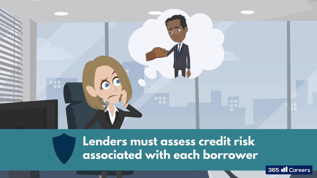
1.2 What is credit risk and why is it important?

5 min

Expected loss (EL) and its components: PD, LGD and EAD

1.3 Expected loss (EL) and its components: PD, LGD and EAD

4 min

Capital adequacy, regulations, and the Basel II accord

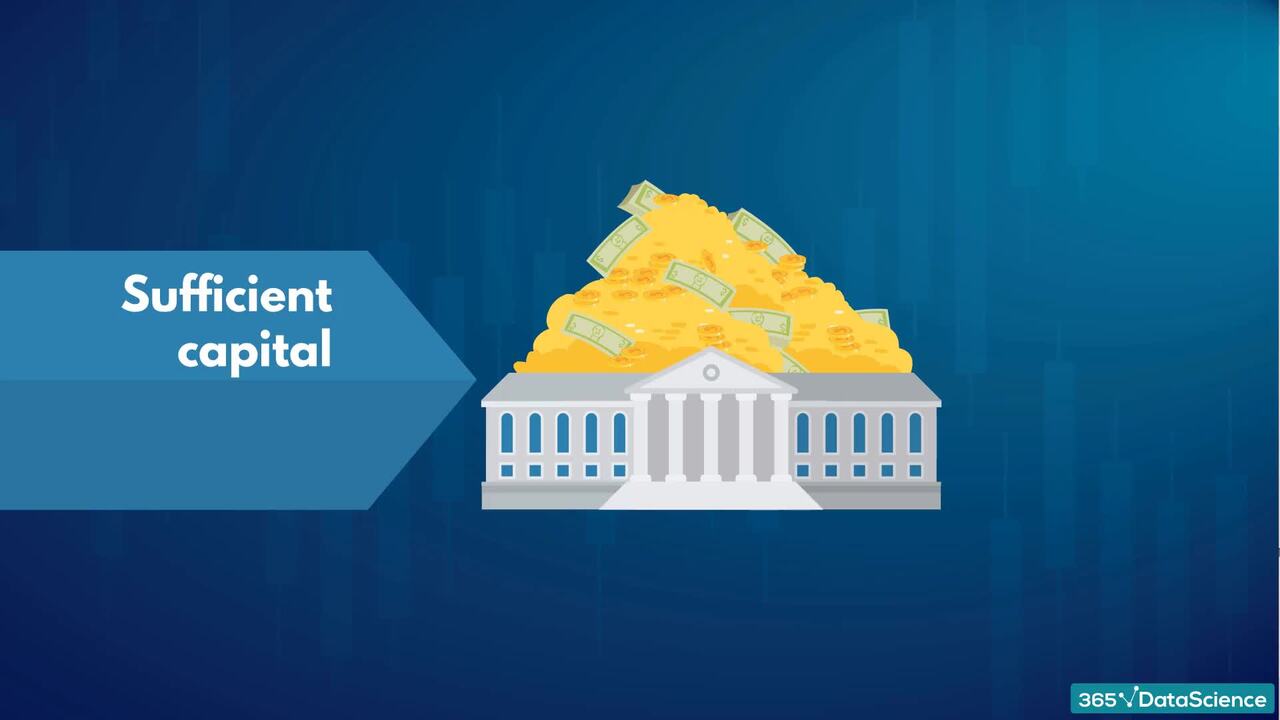
1.4 Capital adequacy, regulations, and the Basel II accord

5 min

Basel II approaches: SA, F-IRB, and A-IRB

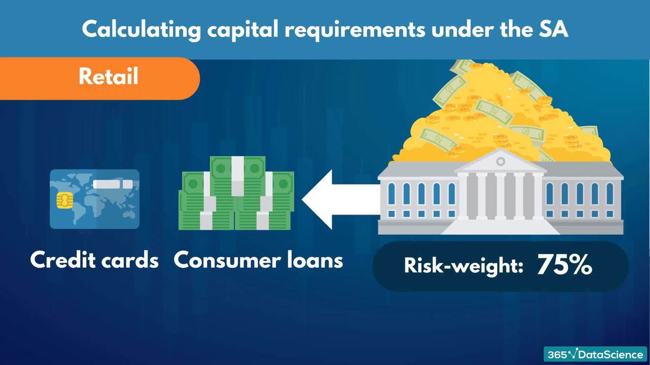
1.5 Basel II approaches: SA, F-IRB, and A-IRB

10 min

Different facility types (asset classes) and credit risk modeling approaches

1.6 Different facility types (asset classes) and credit risk modeling approaches

9 min

Start for free

94%

of AI and data science graduates

successfully change

or advance their careers.

96%

of our students recommend

365 Data Science.

$29,000

average salary increase

after moving to an AI and data science career

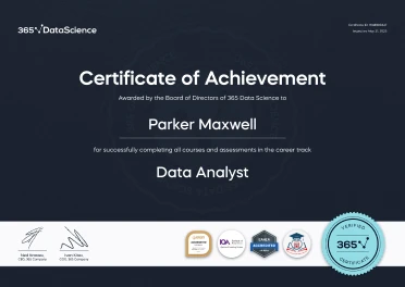
ACCREDITED certificates

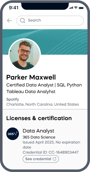
Craft a resume and LinkedIn profile you’re proud of—featuring certificates recognized by leading global institutions.

Earn CPE-accredited credentials that showcase your dedication, growth, and essential skills—the qualities employers value most.

  • Institute of Analytics
  • The Association of Data Scientists
  • E-Learning Quality Network
  • European Agency for Higher Education and Accreditation
  • Global Association of Online Trainers and Examiners

Certificates are included with the Self-study learning plan.

A LinkedIn profile mockup on a mobile screen showing Parker Maxwell, a Certified Data Analyst, with credentials from 365 Data Science listed under Licenses & Certification. A 365 Data Science Certificate of Achievement awarded to Parker Maxwell for completing the Data Analyst career track, featuring accreditation badges and a gold “Verified Certificate” seal.

How it WORKS

  • Lessons
  • Exercises
  • Projects
  • Practice exams
  • AI mock interviews

Lessons

Learn through short, simple lessons—no prior experience in AI or data science needed.

Try for free

Exercises

Reinforce your learning with mini recaps, hands-on coding, flashcards, fill-in-the-blank activities, and other engaging exercises.

Try for free

Projects

Tackle real-world AI and data science projects—just like those faced by industry professionals every day.

Try for free

Practice exams

Track your progress and solidify your knowledge with regular practice exams.

Try for free

AI mock interviews

Prep for interviews with real-world tasks, popular questions, and real-time feedback.

Try for free

Student REVIEWS

A collage of student testimonials from 365 Data Science learners, featuring profile photos, names, job titles, and quotes or video play icons, showcasing diverse backgrounds and successful career transitions into AI and data science roles.