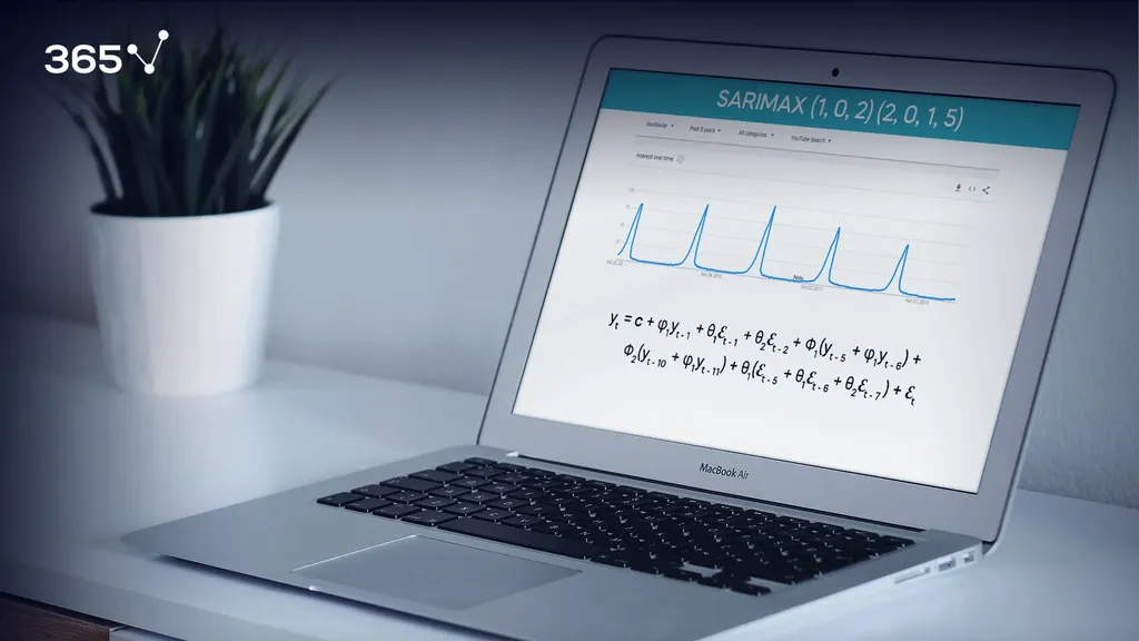
What Is a SARIMAX model? Although we have dedicated a series of blog posts to time series models, we are yet to discuss one very important topic – seasonality.
Each of the models we examined so far – be it AR, MA, ARMA, ARIMA or ARIMAX has a seasonal equivalent.
As you can probably guess, the names for these counterparts will be SARMA, SARIMA, and SARIMAX respectively, with the “S” representing the seasonal aspect.
Therefore, the full name of the model would be Seasonal Autoregressive Integrated Moving Average Exogenous model.
We can all agree that it’s a mouthful, so we’ll stick with the abbreviation.
Additionally, the SARMA and SARIMA can be considered simpler cases of the SARIMAX, where we don’t use integration or exogenous variables, so we’ll mainly focus our attention to the SARIMAX in this tutorial.
What Is Seasonality?
In case you need a hint, seasonality occurs when certain patterns aren’t consistent, but appear periodically. For instance, check out the weekly YouTube searches for Christmas songs like “Jingle Bells”.
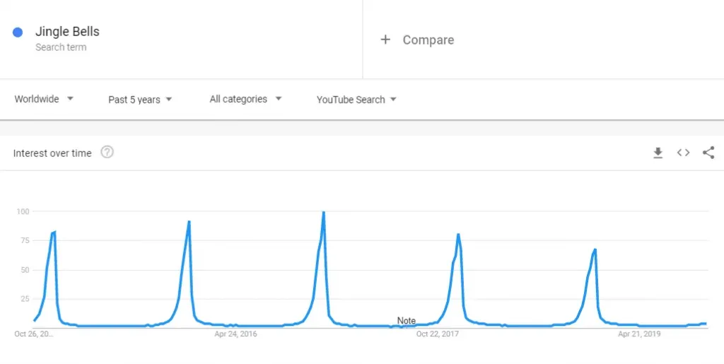
These occur much more frequently over the festive period in December every year. However, the number of times these songs are played is usually a lot lower in June or July.
Therefore, a simple autoregressive component won’t describe the data well.
To elaborate, a simple AR component would severely understate the number of times Christmas songs are played in December, based on the stats from November (1 lag ago). At the same time, it would also greatly overstate the number in January, basing them off of the values recorded in December, since this genre usually experiences a dip after Christmas.
How Do We Handle Seasonality?
To account for such a pattern, we need to include the values recorded during the previous festive period into the model. In this specific example, that would mean relying on the number of times the songs were played last December. Of course, we CAN also include the data from two Decembers back, or even more.

It’s a bit like having another series which is further spread out in time than our original one. Going back to the musical example, the original time series contains values a month apart, while the seasonal one would hold values 12 months apart.

The SARIMAX Model Definition
Now that we’re familiar with the general idea of seasonal models, let’s look at the notation we use and what each value means. Compared to the ARIMAX, the SARIMAX requires 4 additional orders.
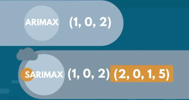
This might sound like a lot, but there’s no need to worry!
The first 3 of these 4 orders are just seasonal versions of the ARIMA orders.
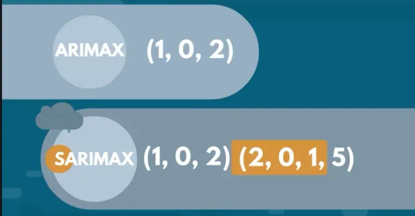
In other words, we have a seasonal autoregressive order denoted by upper-case P, an order of seasonal integration denoted by upper-case D, and a seasonal moving average order signified by upper-case Q. To make differentiation easier, econometricians have agreed to use lower-case letters for their non-seasonal equivalents.
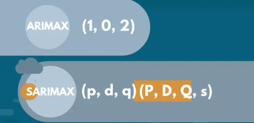
The 4th, and last, order is the length of the cycle. For instance, if we have hourly data, and the cycle length is 24, then the seasonal pattern appears once every 24 hours.
What Is the Length of the Cycle in Seasonal Models?
Another way to think about it is “The number of periods necessary to pass before the tendency reappears”. If we want to inspect a seasonal trend, we need to make sure to set the appropriate cycle length. We represent the last order with a lower-case “s” because it sets the length of each season.
How Do We Interpret Seasonal Orders?
Let’s quickly explain how the 4 new orders work in unison.
Essentially, the length – “s”, - expresses how far away the seasonal components will be from the current period. So, if we have a model with seasonal orders of (2,0,1 and 5), then we’re including the lagged values from 5, and 10 periods ago, as well as the error term from 5 periods ago. Each cycle is “5” periods long and we’re taking 2 lagged seasonal values. So, we’re simply including the values from 5 and 10 periods ago. Similarly, we add the error term from 5 periods ago.

To generalize, we’re interested in every “s”-th value. We start from the “s”-th and go all the way up to “s, times p”. The equivalent is true for seasonal integrated values and seasonal errors as well.

What Is the Equation of a SARIMAX Model?
Let’s see what the equation of a SARIMAX model of order (1,0,1) and a seasonal order (2,0,1,5) looks like.

The interesting part here is that every seasonal component also comprises additional lagged values. If you want to learn why that is so, you can find a detailed explanation of the math behind the SARIMAX model here.
So, what can we see from the equation? The total number of coefficients we are estimating equals the sum of seasonal and non-seasonal AR and MA orders. In other words, we’re looking at a total of “P plus Q, plus, p plus q” – many coefficients.
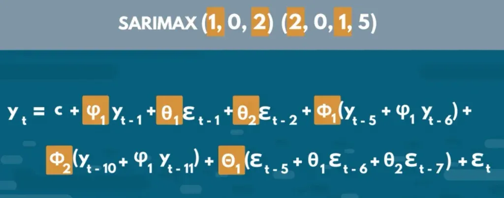
The non-seasonal ones are expressed with lower-case ϕ and θ; while their seasonal counterparts are expressed with upper-case Φ and Θ respectively. Just like with the orders, the capital letters denote the seasonal components and the lower-case ones - the non-seasonal.
So, this is the basic knowledge of seasonal models you need. However, if you want to learn more about time series and time-series data, make sure to check out our article on the topic and enroll in our Time Series Analysis with Python course.
If you’re new to Python, and you’re enthusiastic to learn more, this comprehensive article on learning Python programming will guide you all the way from the installation, through Python IDEs, Libraries, and frameworks, to the best Python career paths and job outlook.

