What is the ARIMAX model?
If you've read our series of blog tutorials on models for estimating time series data, you're already familiar with 3 major approaches - autoregression, moving averages and integration.
What's the common theme in all these models?
They solely relied on a single variable.
However, a model can also take into account more than just past prices or past residuals.
And these are the so-called “MAX” models, with the ARMAX being the non-integrated version and the ARIMAX - its integrated equivalent.
So, in this tutorial, we’re going to explore what they look like and show you how to implement them into Python step-by-step.
Let's get started, shall we?
Why Are ARMAX and ARIMAX Called “MAX” Models?
The names ARMAX and ARIMAX come as extensions of the ARMA and ARIMA respectively. The X added to the end stands for “exogenous”. In other words, it suggests adding a separate different outside variable to help measure our endogenous variable.
The ARMAX and ARIMAX Model Equation:
Since the only difference between the ARMAX and the ARIMAX is that one is integrated and the other one isn’t, we can examine one of them and then highlight how the other one would differ.
We explored an integrated model in our last blog article (ARIMA), so let’s see what the equation of the ARIMAX looks like.
ΔPt =c+βX+ϕ1 ΔPt-1 + θ1 ϵt-1+ϵt
Of course, the equation for the ARMAX would be the same, except we would use the actual variable, say P, instead of its delta.
Pt=c+βX+ϕ1 Pt-1+ θ1 ϵt-1 +ϵt
Breaking Down the ARIMAX Equation:
We can think of the ARMAX as a special case of the ARIMAX, where the order of integration is 0.
So, for the rest of the tutorial, we’ll focus on the ARIMAX.
And we’ll begin by breaking down the different parts in it. For starters, Pt and Pt-1 represent the values in the current period and 1 period ago respectively.
Similarly, ϵt and ϵt-1 are the error terms for the same two periods. And, of course, c is just a baseline constant factor.
The two parameters, ϕ1 and θ1, express what parts of the value Pt-1 and error ϵt-1 last period are relevant in estimating the current one.
Now, the two new additions to the model are “X” and its coefficient β. Just like ϕ, β is a coefficient which will be estimated based on the model selection and the data. But what about X?
What is an exogenous variable?
Well, X is the exogenous variable and it can be any variable we’re interested in.
It can be a time-varying measurement like the inflation rate or the price of a different index. Or a categorical variable separating the different days of the week. It can also be a Boolean accounting for the special festive periods. Finally, it can stand for a combination of several different external factors.
The idea is that it can be any other variable or variables that can affect prices, as long as we have the data available.
Such outside factors are known as exogenous variables in our regression. We use their values to predict and explain the one we’re interested in, which happens to be current prices in our case.
How to Implement ARMAX and ARIMAX Models in Python?
Conveniently enough, the statsmodels package comes in with a method called ARIMA which is fully capable of handling such additional inputs.
We start by specifying the model characteristics and the orders of the model:
![]()
After we’ve done that we also need to specify the exogeneous argument called “exog”.
![]()
The value we want to pass needs to be an array of some sort since we wish to have values associated with every time-period.
For instance, we can use S&P prices as this exogenous variable, since we already have them in our data.
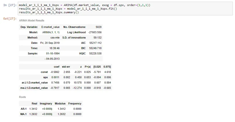
Now, we’re ready to fit an ARIMAX (1,1,1) model.
Make sure to name your model variable in a way that distinguishes it from similar models. In this case, we choose to do this by adding “X, spx” at the end to indicate that the exogeneous variable is the S&P.
Then, as can be seen from the snippets, we set this equal to the ARIMA method as before, we add the time-series, and the order, as we’re used to. Finally, between the two, we set the “exog” argument equal to “DF SPX”, which indicates the S&P prices.
![]()
If we fit this model and print its summary table, we’re going to see that we get an additional row for the S&P prices.

And that’s all there is to it!
We’ve successfully seen how to implement an ARIMAX model in Python.
If you want to learn more about ARIMAX and other time series models in Python, make sure to enroll in our Time Series Analysis with Python course.
Ready to take the next step towards a career in data science?
Check out the complete Data Science Program today. Start with the fundamentals with our Statistics, Maths, and Excel courses. Build up a step-by-step experience with SQL, Python, R, Power BI, and Tableau. And upgrade your skillset with Machine Learning, Deep Learning, Credit Risk Modeling, Time Series Analysis, and Customer Analytics in Python. Still not sure you want to turn your interest in data science into a career? You can explore the curriculum or sign up for 15 hours of beginner to advanced video content for free by clicking on the button below.


