Nothing is set in stone in the world of finance. Whether you are managing a company or investing your savings, you have to carefully consider all the moving parts when making any decision about money! Thankfully, there are tools that you can use to apply data science in finance in a straightforward and stress-free way.
Monte Carlo simulations do just that. They are widely used in corporate finance, investment valuation, asset management, risk management, estimating insurance liabilities, pricing of options, and other derivatives.
In this article, we’ll explain the mechanics of Monte Carlo simulation, and see how it can be used for standard financial analysis.
What Is Monte Carlo Simulation?
Any action or decision we perform in the world can have a number of outcomes that depend on factors beyond our control. What a Monte Carlo simulation does is consider likely variations in the circumstances surrounding an event to try and predict its results.
In other words, when we run a Monte Carlo simulation, we are interested in observing the different possible realizations of a future event. We can use past data, something we already know, to create a simulation – a new set of fictional but sensible data.
These realizations are generated by observing the distribution of the historical data and calculating its mean and variance. The mean, or simple average, of a dataset, is calculated by adding up all of its components and then dividing them by the number of components contained in the dataset. On the other hand, variance measures the dispersion of a set of data points around their mean value. Such information is valuable, as it allows us to consider a good proxy of the probability of different outcomes and can help us make an informed decision.
To see our analysis through, we will also need two more statistical terms – standard deviation and normal distribution. Both appear later in this article so you might want to read up on them before we proceed!
Monte Carlo Simulation in Finance
Now, imagine you are a finance manager, and you want to gain insight into the direction your company is headed. To estimate the current year revenues, you would use this simple equation:
\[ Current\: Revenues = Last\: Year\: Revenues \times (1 + YoY\: Growth\: Rate) \]
The two parameters you need, revenue growth and standard deviation, could be obtained by looking at historical figures or arbitrarily chosen, based on the user’s intuition.
The reasoning for Cost of Goods Sold (COGS) and Operating expenses (Opex) is almost the same, with one main difference. We need to represent COGS and Opex as a percentage of revenues, then model the development of the percentage of revenues.
When you deduct COGS from the revenue of a company, you will obtain its gross profit.
Monte Carlo Simulation in Python: Example
Let’s see how we can utilize a Monte Carlo computer simulation to prepare our financial forecast. To do this, you will need a basic understanding of how Python works. We’ll also be using the Jupyter Notebook, so it’s advisable to refresh your knowledge of it as well.
As we said, our goal is to predict the firm’s future gross profit. We will need the values of expected revenue and expected cost of goods sold.
First, let’s import the two main tools that will help us with the Monte Carlo analysis: NumPy and Matplotlib Py-plot.
import numpy as np
import matplotlib.pyplot as plt
Part 1: Expected Revenues
For the first part of our Monte Carlo simulation example, we’ll perform 1,000 simulations of the company’s expected revenues.
Assume you have considered last year’s revenue and you have an idea about the revenue growth rate you can expect, so the expected revenues for this year are \$170 million, and a standard deviation of this figure would be \$20 million.
Therefore, assign 170 to a variable “rev_m”, standing for “revenue mean”, and 20 to a variable “rev_stdev”, standing for “revenue standard deviation”.
The next important value we need to specify is the number of iterations. We intend to produce 1,000 simulated observations from a normal distribution. So, in a variable called “iterations”, record the value 1,000.
rev_m = 170
rev_stdev = 20
iterations = 1000
The next line of code will produce the simulation of future revenues.
We will apply NumPy’s random normal distribution generator. The arguments we have here are the expected mean of revenues, their standard deviation, and the number of iterations we would like to perform.
We will store this information in a variable, called “rev”. The outcome will be 1,000 values, most of which are close to the mean we selected.
rev = np.random.normal(rev_m, rev_stdev, iterations)
rev
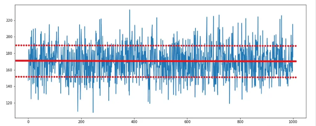
Let’s plot these observations and see their distribution:
plt.figure(figsize=(15, 6))
plt.plot(rev)
plt.show()
The simulated values are centered on the mean of 170. It is obvious that almost all data points fall in the region of 150 to 190. The two values equal the mean minus one standard deviation and the mean plus one standard deviation. For 1,000 data points, we rarely observe scenarios outside of these limits.
Part 2: Estimating COGS
For the second part of our Monte Carlo simulation example, we’ll try to estimate the cost of goods sold (COGS)
Assume you are experienced in this business and able to tell that, typically, COGS amount to approximately 60% of the company’s annual revenues. 60% of its revenues are spent to produce the goods it sells. And what do we mean by approximately?
Well, if the past COGS values were once equal to 55% of revenue, and then 62%, 63%, and finally 55% again, you may reasonably consider a normal distribution with a mean of 60% of revenues, and the estimation of 60% will have a standard deviation of 10%. It does not matter that COGS was deviating with 6% of the revenue value. For setting the distribution, it should deviate 10% regarding the mean of COGS.
Here is how we can type this in Python. COGS are money spent; therefore, we should put a minus sign first. Then, the expression must reflect the multiplication of revenues by 60%.
We will not simulate COGS 1,000 times. This has already been done for revenues, and we have 1,000 revenue data points. We must assign a random COGS value to each one of these points. COGS are a percentage of revenues. Therefore, the revenue value we obtained must be multiplied by a value extracted from a random normal distribution, with a mean of 0.6 and a standard deviation of 0.1.
COGS = - (rev * np.random.normal(0.6,0.1))

plt.figure(figsize=15, 6))
plt.plot(COGS)
plt.show()
Part 3: Calculating Gross Profit
For the final part of our Monte Carlo simulation example, we’ll calculate gross profit.
Since we have generated 1,000 potential revenue and COGS values, calculating the simulation of gross profit requires us to combine the revenue and COGS (which we created as a negative number, so it is correct to use a plus and not a minus sign here!).
Gross_Profit = rev + COGS
Gross_Profit

plt.figure(figsize=(15, 6))
plt.plot(Gross_Profit)
plt.show()
From this moment, with the help of the max and min functions, it is straightforward to obtain the biggest and the smallest potential value of gross profit. The methods “mean” and “STD” can provide an output equal to the mean and the standard deviation of the gross profit, respectively.
Monte Carlo Simulation: Example Results
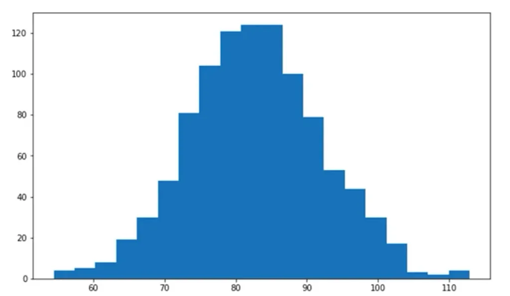
Let’s visualize the results of our Monte Carlo simulation example!
You can take your analysis even further with the use of histograms, a popular data visualization tool. The syntax to implement it is identical to the one we used for a regular plot, but the difference is that, on the second line after “plt”, you need to type “hist”. Then, you could add many arguments, but two are important. One of them is the value of interest, which, in our case, is gross profit. The other one regards the bins. These are the chunks in which the data in the plot will be divided.
plt.figure(figsize=(10, 6));
plt.hist(Gross_Profit, bins = 20);
plt.show()
This is how Monte Carlo Simulation is used in standard financial analysis. Our Python for Finance course covers these and more sophisticated procedures in depth. Estimating a firm’s share price and EBIT or pricing stock options are all required skills for data scientists working in the financial sector and mastering them can boost your job prospects tremendously!
Are you ready for the next step toward a career in data science?
The 365 Data Science Program offers self-paced courses led by renowned industry experts. Starting from the very basics all the way to advanced specialization, you will learn by doing with a myriad of practical exercises and real-world business cases. If you want to see how the training works, start with our free lessons by signing up below.


