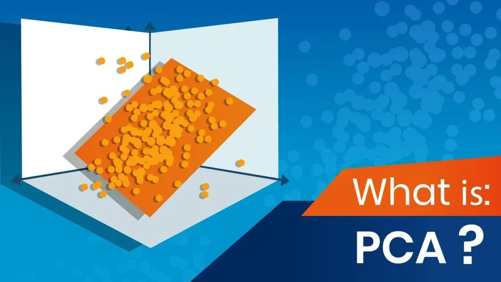
Principal Components Analysis or PCA is a popular dimensionality reduction technique you can use to avoid “the curse of dimensionality”.
But what is the curse of dimensionality? And how can we escape it?
The curse of dimensionality isn’t the title of an unpublished Harry Potter manuscript but is what happens if your data has too many features and possibly not enough data points. In order to avoid the curse of dimensionality one can employ dimensionality reduction.
So, in this article, we’ll take a close look at dimensionality reduction and Principal Components Analysis.
We’ll talk about Principal Component Analysis definition, its practical application, and how to interpret PCA. By the end of the article, you’ll be able to perform a Principal Component Analysis yourself.
Sound good?
Let’s get started. The first question of the day is:
What Is Dimensionality Reduction?
Imagine we have a dataset with 3-variables. Visually, our data may look like this:
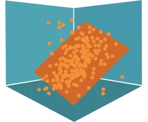
Now, in order to represent each of those points, we have used 3 values – one for each dimension.
And here comes the interesting part.
In some cases, we can find a 2D plane very close to the data. Something like this:
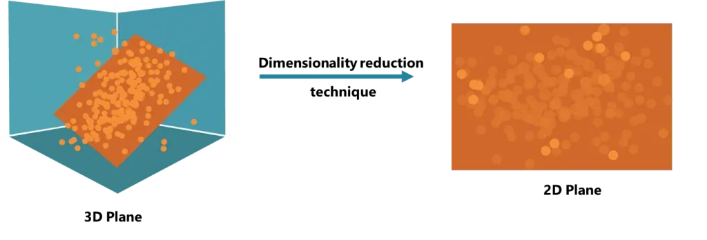
This plane is two-dimensional, so it is defined by two variables. As you can see, not all points lie on this plane, but we can say that they approximately do.
Linear algebraic operations allow us to transform this 3-dimensional data into 2-dimensional data. Of course, some information is lost, but the total number of features is reduced.
In this way, instead of having 3 variables, we reduce the problem to 2 variables.
In fact, if you have 50 variables, you can reduce them to 40, or 20, or even 10. And that’s where dimensionality reduction has the biggest impact.
How Does Dimensionality Reduction Work in the Real World?
Well, imagine a survey where there is a total of 50 questions. Three of them are the following: Please rate from 1 to 5:
- I feel comfortable around people
- I easily make friends
- I like going out
Now, these questions may seem different.
But here’s a catch.
In the general case, they aren’t. They all measure your level of extroversion. So, it makes sense to combine them, right? That’s where dimensionality reduction techniques and linear algebra come in! Very, very often we have too many variables that are not so different, so we want to reduce the complexity of the problem by reducing the number of variables.
And that’s the gist of dimensionality reduction.
And it just so happens that PCA is one of the simplest and most widely used methods in this area.
Why Do We Use Principal Components Analysis?
You might be interested to discover that PCA dates all the way back to the early work of Pearson in 1901. Nowadays, however, it’s commonly used in preprocessing. PCA is often employed prior to modeling and clustering, in particular, to reduce the number of variables.
To define it more formally, PCA tries to find the best possible subspace which explains most of the variance in the data. It transforms our initial features into so-called components. These components are basically new variables, derived from the original ones, and they are usually displayed in order of importance. At the end of the PCA analysis, we aim to choose only a few components, while preserving as much of the original information as possible.
Now I know what you’re thinking: this sounds highly theoretical. But don’t worry.
I’ll walk you through the practical side of PCA, which will make the concept clearer.
How Does Principal Components Analysis Work?
Practice makes perfect, so let’s see how to implement a practical Principal Component Analysis example in Python using sk learn.
Let’s say we have a data set, containing information about customers.
The first thing we’ll need to do in Python is read the file.

Now, we can take a look at the data. It contains 7 geo-demographical features about customers and their IDs.

We have information about age, income and education level, among others.
Our goal will be to use a PCA algorithm to reduce the number of these 7 features to a smaller number of principal components. So, the next step is to import the relevant module for PCA from sk learn: 
We can directly use the PCA method, provided by the sk learn library. We can create an instance of the PCA class and then simply apply the fit method to the PCA variable with the PCA data as an argument.

And that’s all you need to successfully obtain your PCA data.
How to Interpret Principal Components Analysis?
Now, PCA essentially creates as many principal components as there are features in our data, in our case 7. Moreover, these components are arranged in order of importance. In case you’re wondering, importance here indicates how much of the PCA variance of our data is explained by each component.
Now that we’ve clarified that, we can call the ‘explained variance ratio’ attribute to actually check what happened.

We can see that there are 7 components. In essence, PCA applied a linear transformation on our data, which created 7 new variables. Now, some of them contain a large proportion of the variance, while others – almost none. Together these 7 components explain 100% of the variability of the data – that’s why if you sum up all the numbers you see, you’ll get 1.
We observe that the first component explains around 36% of the variability of the data, the second one: 26%, the third: 19% and so on. And the last component explains only 2% of the information.
So, our task now will be to select a subset of components while preserving as much information as possible.
Logically, we want to include the most prominent components. Therefore, if we want to choose 2 components, we would choose the first 2, as they contain most of the variance. If we opt for 3, we would take the first 3 and so on.
A very useful graph here would be a line chart that shows the cumulative explained variance against the number of components chosen.
So, the next step in the analysis is to plot the number of components that we can choose so that 1 to 7 appear on the x-axis and the cumulative explained variance ratio on the y-axis. To achieve the latter, we simply take the respective attribute and apply the ‘cumulative sum’ method on it.
This is the relevant code to achieve it:

And here is the variance of PCA plot:
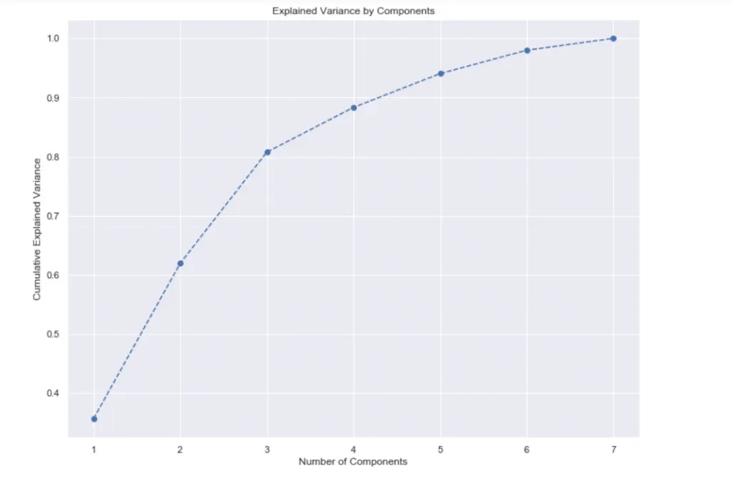
Now that we can see the explained variance by number of components, we can take a look at our PCA plot and analyse the results.
This visual is not only important but is actually quite handy. It will help us decide how many components to keep in our dimensionality reduction. If we choose 2 components, we can see that we preserve around 60% of the information. If we choose 3 components – around 80%. With 4 of them, we’ll keep almost 90% of the initial variability.
So how do we actually choose the number of components? Well, there is no right or wrong answer. A rule of thumb is to keep at least 70-80% of the explained variance. As mentioned, if we take all 7, we would have 100% of the information, but we wouldn’t reduce the dimensionality of the problem at all.
In this case, keeping 3 or 4 components makes sense. Both options would reduce our features significantly while preserving most of the information. Having 3 components means we’ll preserve over 80 % of the variance in this case, so this is what we’ll land on.
Finally, we must write the relevant code to keep only 3 components.
We’ll use the same class again, PCA, and specify the desired number of components as an argument. In the end, we fit the PCA with the standardized data once again.

And that’s it! Simple as that, we have performed Principal Components Analysis. The next step in Principal Component Analysis is the interpretation of the components and the principal components scores. But that’s a tale for another time.
Let’s recap:
PCA is widely used in machine learning as a dimensionality reduction technique. You can think of it as your Patronus against the forces of high dimensional and sparse data. If you don’t know what a Patronus is, I congratulate you on having a life, I guess. In any case, you now know what PCA is (and I hear that’s more frequently asked during data science interviews).
Eager to learn more? Check out the 365 Customer Analytics Course in our Data Science Training. If you still aren’t sure you want to turn your interest in data science into a career path, we also offer a free preview version of the Data Science Program. You’ll receive 12 hours of beginner to advanced content for free. It’s a great way to see if the program is right for you.


