We all know Coca-Coca, the conglomerate giant. The company makes millions of dollars each year and can seemingly anticipate every issue or new market trend. However, have you ever thought about how they stay on top of the game? It’s because their data science teams use time series analysis.
In this article, we’ll explore what this technique entails through real-world examples, and discuss the types of time series modeling you’re likely to encounter.
What Is Time Series Analysis?
In a management context, we are typically interested in forecasting certain types of outcomes. Some examples are sales (at a total or a division level), customer satisfaction levels, the company’s ability to achieve target cost levels, or capability to deliver successful projects. In all these cases, we’ll use past data to come up with a prediction about the future. Time series analysis is part of predictive analysis, gathering data over consistent intervals of time (a.k.a. collecting time series data). It’s an effective tool that allows us to quantify the impact of management decisions on future outcomes.
Let’s take Coca-Cola again and look at a time series analysis example through the lens of the company’s sales. Two quarters from now, their expected sales will be anywhere between 250,000 and 300,000 units. Historical sales indicate a strong relationship between unit sales and weather – otherwise known as correlation analysis. Based on that, it is likely that the numbers will be closer to 290,000 in the summer months. However, to achieve similar results in the winter quarter, the company will need some additional marketing investments.
The technique the Coca-Cola team can use to perform this type of future forecasting is precisely time series analysis. When applied, the model will provide a range of potential outcomes. In our example, the variable we are interested to predict is future sales volume. Therefore, the outcomes will vary depending on numerous factors, which may affect sales development throughout the year.
Let’s suppose the weather is 5% warmer than average, and Coca-Cola spend 5% more on marketing by investing in TV ads and promotional events. Then, based on historical data, we can reasonably expect that sales will be on the higher end of the range we indicated - 290,000 units. By changing the weather condition assumptions and running hypothesis testing on different marketing spend, the model would yield a separate time series analysis forecast. Typically, in practice, we will provide a range of estimates. For Coca-Cola, they might look something like this:
- 290,000 units in the best-case scenario
- 250,000 units in the worst-case scenario
- 270,000 in a base-case scenario
What Are the Types of Time Series Modelling Methods?
There are 4 modeling methods that analysts often use to support time series analysis:
- Naive
- Probabilistic
- Deterministic
- Hybrid
We’ll now explore each type and give you examples of how to apply them in a business setting.
Naive Time Series Method
A naive forecast – or persistence forecast – is the simplest form of time series analysis where we take the value from the previous period as a reference:
\[x_t = x_{t+1}\]
It does not require large amounts of data – one data point for each previous period is sufficient. Additionally, naive time series modeling can take seasonality and trend into account.
If you recall the Coca-Cola example, seasonality suggests that there is a cyclical pattern in the data that only appears periodically. Instead of taking the sales volume for the previous month, you can take last year’s value for the same month you’re trying to predict now:
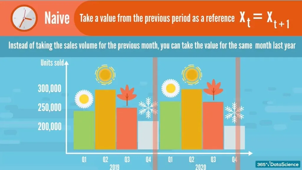
In essence, you would be using last December’s numbers, instead of this November’s values, to forecast the sales for this upcoming December.
Another option is to consider the trend. For example, based on our historical analysis, we can see that last year’s September sales dropped 10% versus those made in August. We can use this information to forecast September of this year by applying the 10% reduction of sales versus the August ones:
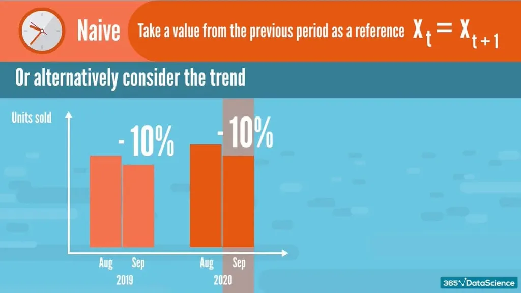
The naive forecasting method is easy to understand and to use. However, the past is not always a good indicator of the future. That is why more sophisticated analytical techniques are often required to come up with more accurate sales forecasts.
Probabilistic Time Series Method
Probabilistic modeling is also known as a Monte Carlo simulation. It’s named after the gambling hot spot in Monaco as it simulates real-life events with uncertain outcomes.
When faced with significant uncertainty, the Monte Carlo Simulation allows you to use a range of input values rather than just replacing the uncertain variable with a number. More precisely, these input values make use of the variable’s distribution function and help obtain a large number of possible realizations of the output variable.
To illustrate, here is an example of a Monte Carlo simulation for a revenue forecast:
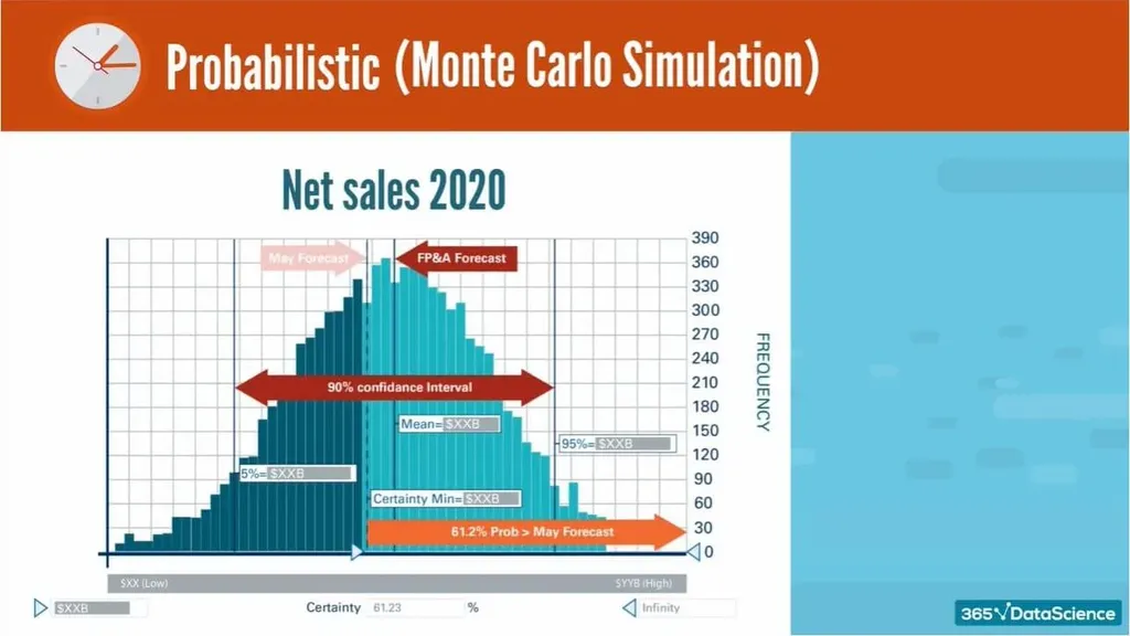
There is a 90% chance that total revenue will be between X and Y, and a 61.2% chance that the service will be higher than the forecast.
The advantage of Monte Carlo simulation is that it fully explores the probability distribution function of a certain variable. In our example, that’s the development of sales. Fortunately, we are able to study the probability of the sales that will fall within a certain bandwidth. Knowing this will help us manage risk.
However, to be successful, we need reliable data. If we do a Monte Carlo simulation and obtain no certainty that sales will fall within a specific bandwidth, then the probabilistic modeling has no added value.
Deterministic Time Series Method
The third method we’ll be looking at is the deterministic model – a more complex form of time series analysis that includes user-defined confidence intervals. As an example, let’s examine a historical trend and a forecast with a certain level of confidence for the year to come:
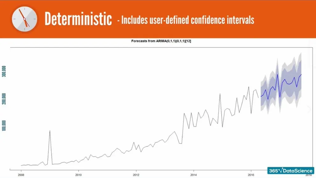
Suppose we want to see the sales forecast within a 95% range of certainty. Then, based on the graph, we can say with 95% certainty that we expect sales to be in the region from 240,000 to 280,000 units.
In other words, we provide an interval based on a deterministic trend, instead of making a definitive claim that we will make 265,000 sales. Thus, we have a better chance of preparing for the future because we know what the best- and worst-case scenarios look like.
Hybrid Time Series Method
The last type of time series analysis we will discuss is called hybrid modeling. As the name suggests, it combines two other types of models - probabilistic and deterministic. The hybrid model considers the available data, then steps on it to simulate how uncertainties can affect the output.
For example, suppose we increase our marketing budget whilst having similar weather as last year. Then, we can expect a sales volume between 240,000 and 280,000 units with 90% certainty:
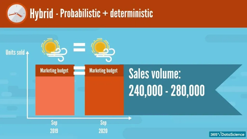
This is a multi-step process, so we don’t get these numbers right away. Instead, we first go with the deterministic approach to find a model which describes the data well. In most cases, this is some variation of an ARIMA model: $x = \alpha + \beta_1 x_{t-1} + \beta_2 x_{t-1}$ , etc.
Then, we expand it to include a trend or a seasonal component based on some manual analysis. After we find the best fitting model, we conduct a Monte Carlo simulation to see how a random variable with the same statistical parameters would evolve over time. Of course, the simulation conducts this forecast thousands of times. At the end of it, we get a range of the most frequently predicted values to create our 90% confidence interval.
Overall, we can say that hybrid modeling is the most popular approach as it combines two types of methods to give us the highest percentage of certainty possible.
Time Series Analysis: What’s Next?
Time series analysis brings exponential value to business development. Analysts utilize it to help companies estimate their revenue, predict trends, and future-proof their products.
As this type of analysis is part of business analytics, having it in your tool box means that you will be at a vital position in a company which offers heaps of career growth opportunities.


