Exploring the 5 OLS Assumptions for Linear Regression Analysis

If this is your first time hearing about the OLS assumptions, don’t worry. If this is your first time hearing about linear regressions though, you should probably get a proper introduction. In the linked article, we go over the whole process of creating a regression. Furthermore, we show several examples so that you can get a better understanding of what’s going on. One of these is the SAT-GPA example.

Linear Regression Example

To sum up, we created a regression that predicts the GPA of a student based on their SAT score.

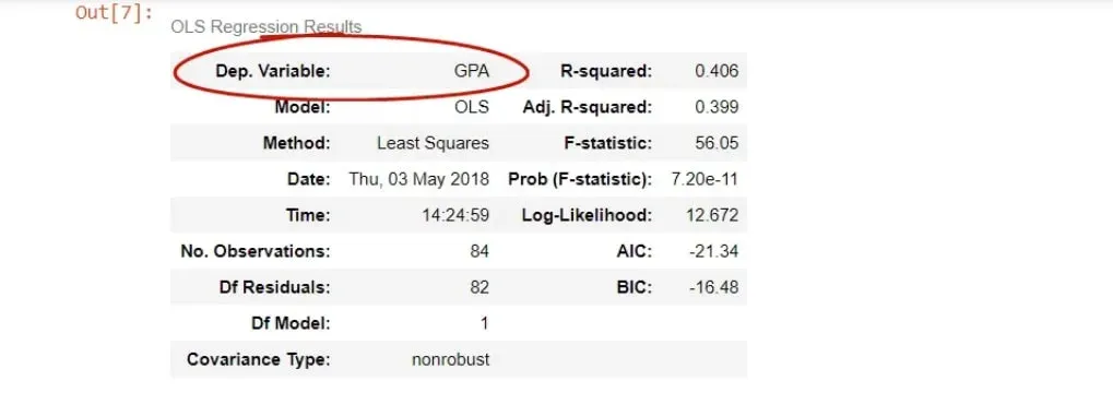
Below, you can see the table with the OLS regression tables, provided by statsmodels.

Some of the entries are self-explanatory, others are more advanced. One of them is the R-squared, which we have already covered.

Now, however, we will focus on the other important ones.

First, we have the dependent variable, or in other words, the variable we are trying to predict.

As you can tell from the picture above, it is the GPA. Especially in the beginning, it’s good to double check if we coded the regression properly through this cell.

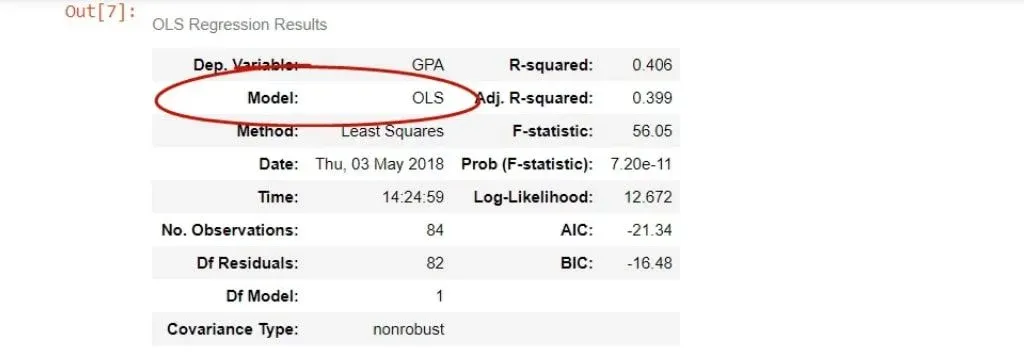
After that, we have the model, which is OLS, or ordinary least squares.

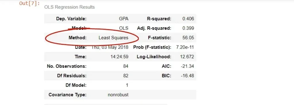
The method is closely related – least squares.

In this case, there is no difference but sometimes there may be discrepancies.  

What Is the OLS

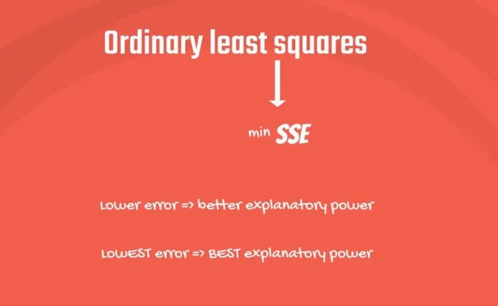
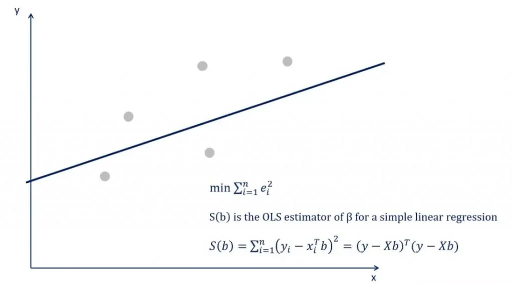
OLS, or the ordinary least squares, is the most common method to estimate the linear regression equation. Least squares stands for the minimum squares error, or SSE.

You may know that a lower error results in a better explanatory power of the regression model. So, this method aims to find the line, which minimizes the sum of the squared errors.

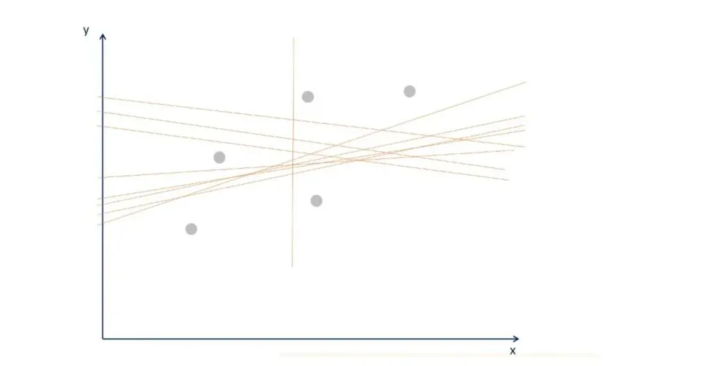
Let’s clarify things with the following graph.

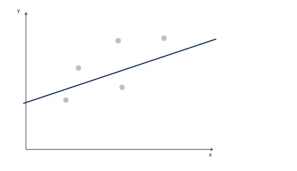
You can tell that many lines that fit the data. The OLS determines the one with the smallest error. Graphically, it is the one closest to all points, simultaneously.

The Formula

The expression used to do this is the following.

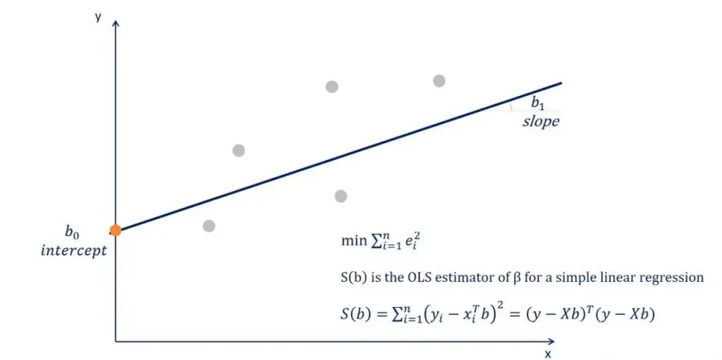
But how is this formula applied? Well, this is a minimization problem that uses calculus and linear algebra to determine the slope and intercept of the line. After you crunch the numbers, you’ll find the intercept is b₀ and the slope is b₁.

Knowing the coefficients, here we have our regression equation.

Minimizing the SSE

We can try minimizing the squared sum of errors on paper, but with datasets comprising thousands of values, this is almost impossible.

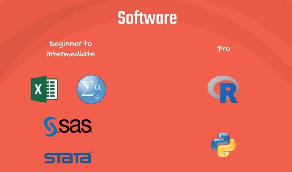
Nowadays, regression analysis is performed through software. Beginner statisticians prefer Excel, SPSS, SAS, and Stata for calculations. Data analysts and data scientists, however, favor programming languages, like R and Python, as they offer limitless capabilities and unmatched speed. And that’s what we are aiming for here!

Alternative Methods to the OLS

Finally, we must note there are other methods for determining the regression line. They are preferred in different contexts.

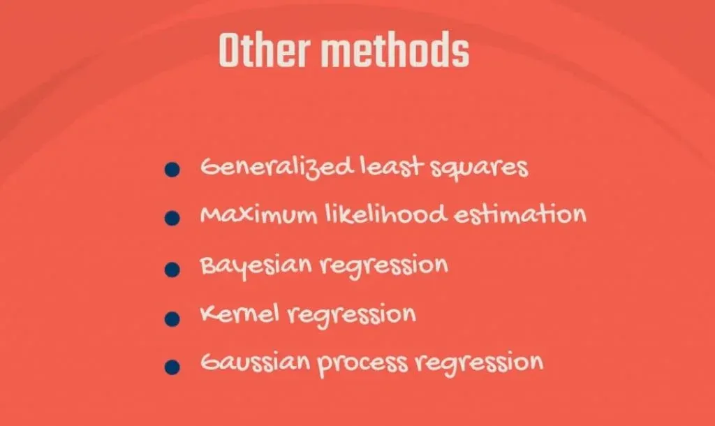
Such examples are the Generalized least squares, Maximum likelihood estimation, Bayesian regression, the Kernel regression, and the Gaussian process regression.

However, the ordinary least squares method is simple, yet powerful enough for many, if not most linear problems.

The OLS Assumptions

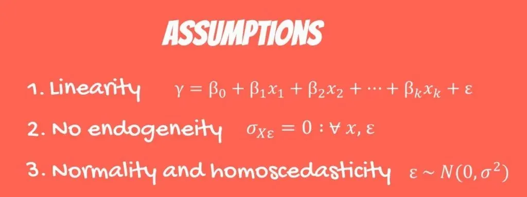
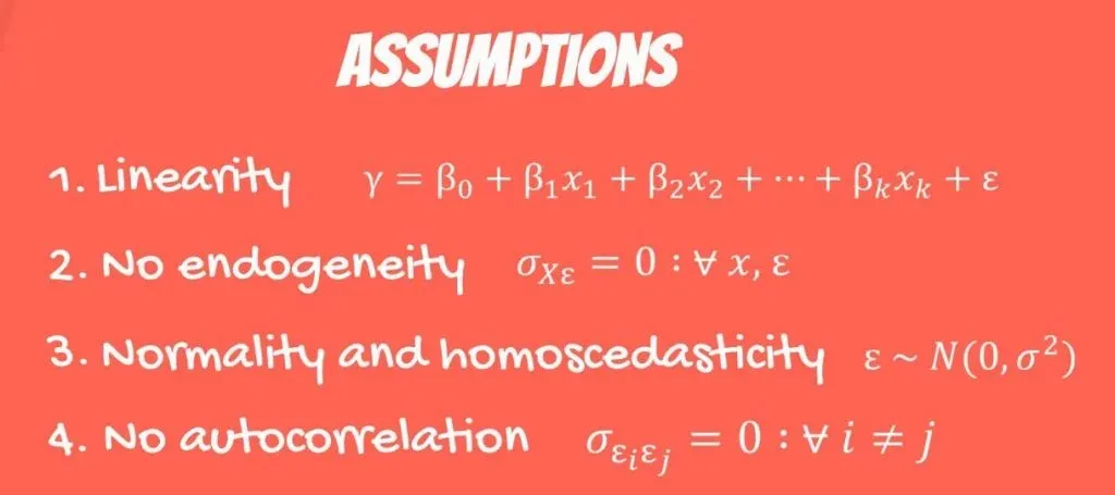
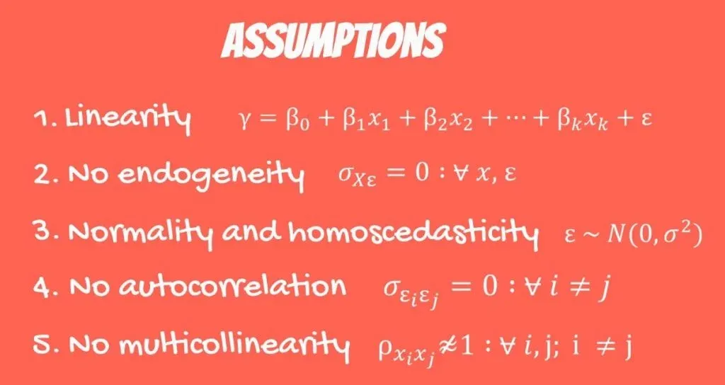
So, the time has come to introduce the OLS assumptions. In this tutorial, we divide them into 5 assumptions. You should know all of them and consider them before you perform regression analysis.

The First OLS Assumption

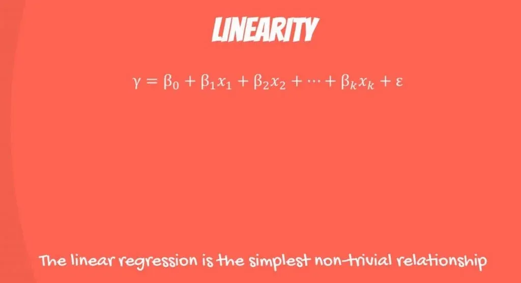
The first one is linearity. It is called a linear regression. As you may know, there are other types of regressions with more sophisticated models. The linear regression is the simplest one and assumes linearity. Each independent variable is multiplied by a coefficient and summed up to predict the value.

The Second OLS Assumption

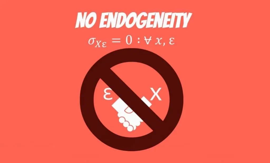
The second one is endogeneity of regressors. Mathematically, this is expressed as the covariance of the error and the Xs is 0 for any error or x.

The Third OLS Assumption

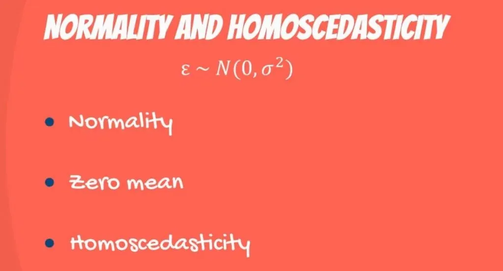
The third OLS assumption is normality and homoscedasticity of the error term. Normality means the error term is normally distributed. The expected value of the error is 0, as we expect to have no errors on average. Homoscedasticity, in plain English, means constant variance.

The Fourth OLS Assumption

The fourth one is no autocorrelation. Mathematically, the covariance of any two error terms is 0. That’s the assumption that would usually stop you from using a linear regression in your analysis.

The Fifth OLS Assumption

And the last OLS assumption is no multicollinearity. Multicollinearity is observed when two or more variables have a high correlation between each other.

These are the main OLS assumptions. They are crucial for regression analysis. So, let’s dig deeper into each and every one of them.

OLS Assumption 1: Linearity

The first OLS assumption we will discuss is linearity.

As you probably know, a linear regression is the simplest non-trivial relationship. It is called linear, because the equation is linear.

Each independent variable is multiplied by a coefficient and summed up to predict the value of the dependent variable.

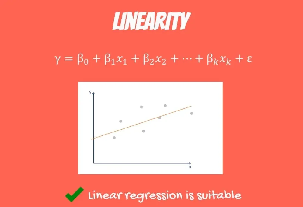
How can you verify if the relationship between two variables is linear? The easiest way is to choose an independent variable X₁ and plot it against the depended Y on a scatter plot. If the data points form a pattern that looks like a straight line, then a linear regression model is suitable.

An Example Where There is No Linearity

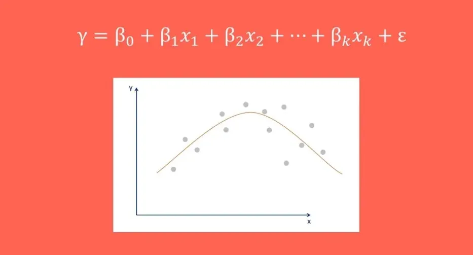
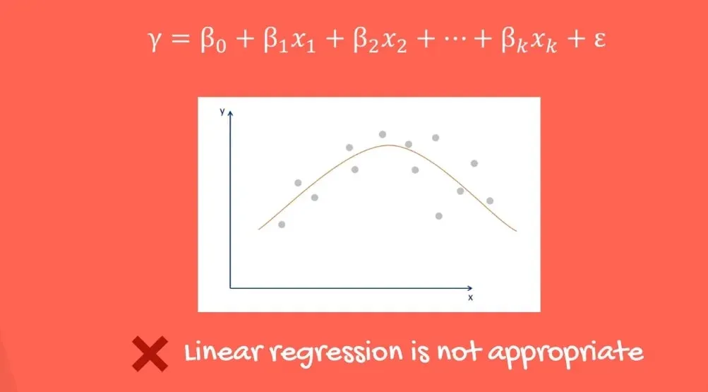
Let’s see a case where this OLS assumption is violated. We can plot another variable X₂ against Y on a scatter plot.

As you can see in the picture above, there is no straight line that fits the data well.

Actually, a curved line would be a very good fit. Using a linear regression would not be appropriate.

Fixes for Linearity

Linearity seems restrictive, but there are easy fixes for it. You can run a non-linear regression or transform your relationship. There are exponential and logarithmical transformations that help with that. The quadratic relationship we saw before, could be easily transformed into a straight line with the appropriate methods.

Important: The takeaway is, if the relationship is nonlinear, you should not use the data before transforming it appropriately.

OLS Assumption 2: No Endogeneity

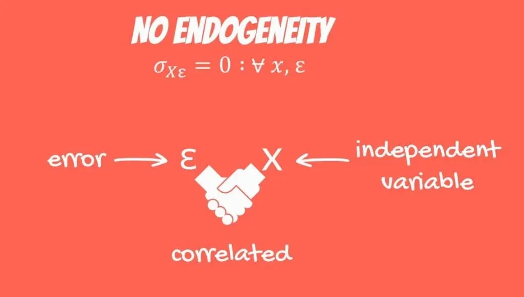
The second OLS assumption is the so-called no endogeneity of regressors. It refers to the prohibition of a link between the independent variables and the errors, mathematically expressed in the following way.

Think about it. The error is the difference between the observed values and the predicted values. In this case, it is correlated with our independent values.

Omitted Variable Bias

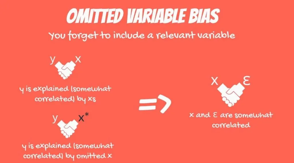
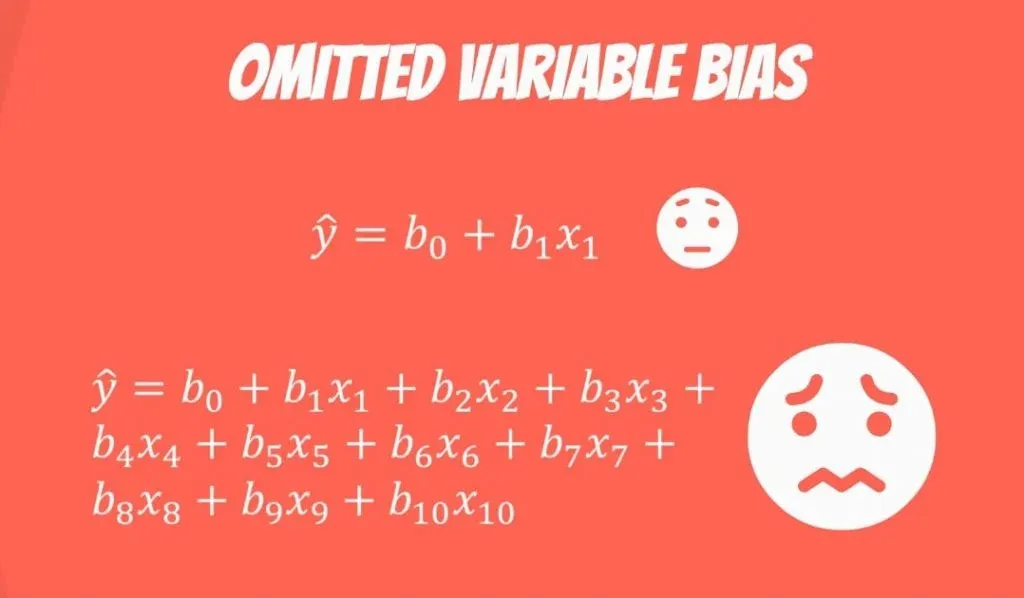
This is a problem referred to as omitted variable bias. Omitted variable bias is introduced to the model when you forget to include a relevant variable.

As each independent variable explains y, they move together and are somewhat correlated. Similarly, y is also explained by the omitted variable, so they are also correlated. Chances are, the omitted variable is also correlated with at least one independent x. However, you forgot to include it as a regressor.

Everything that you don’t explain with your model goes into the error. So, actually, the error becomes correlated with everything else.

A Case in Point

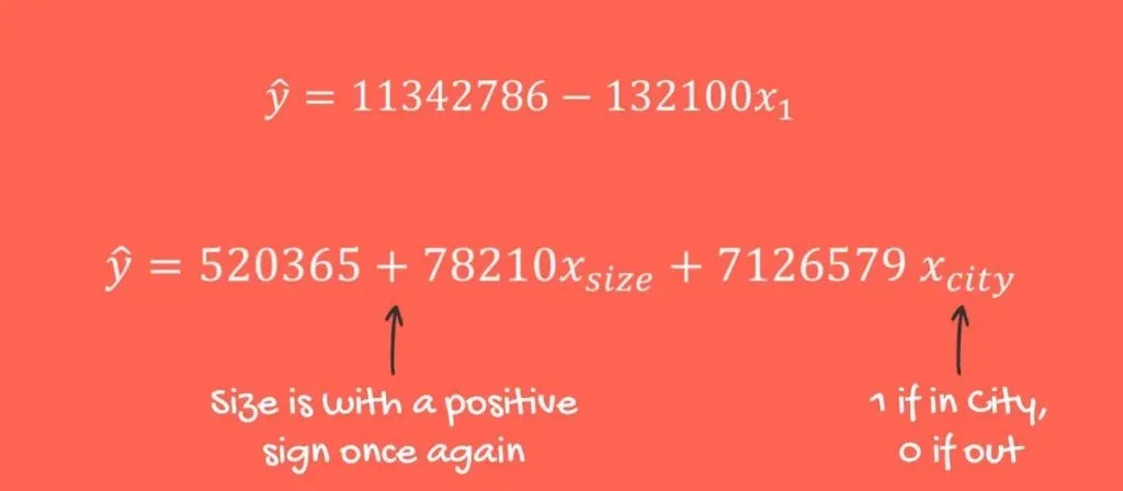
Before you become too confused, consider the following. Imagine we are trying to predict the price of an apartment building in London, based on its size. This is a rigid model, that will have high explanatory power.

However, from our sample, it seems that the smaller the size of the houses, the higher the price.

This is extremely counter-intuitive. We look for remedies and it seems that the covariance of the independent variables and the error terms is not 0. We are missing something crucial.

Fixing the Problem

Omitted variable bias is hard to fix. Think of all the things you may have missed that led to this poor result. We have only one variable but when your model is exhaustive with 10 variables or more, you may feel disheartened.

Critical thinking time. Where did we draw the sample from? Can we get a better sample? Why is bigger real estate cheaper?

Getting More Information

The sample comprises apartment buildings in Central London and is large. So, the problem is not with the sample. What is it about the smaller size that is making it so expensive? Where are the small houses? There is rarely construction of new apartment buildings in Central London. And then you realize the City of London was in the sample.

The place where most buildings are skyscrapers with some of the most valuable real estate in the world. If Central London was just Central London, we omitted the exact location as a variable. In almost any other city, this would not be a factor. In our particular example, though, the million-dollar suites in the City of London turned things around.

Let’s include a variable that measures if the property is in London City. As you can see in the picture below, everything falls into place.

Larger properties are more expensive and vice versa.

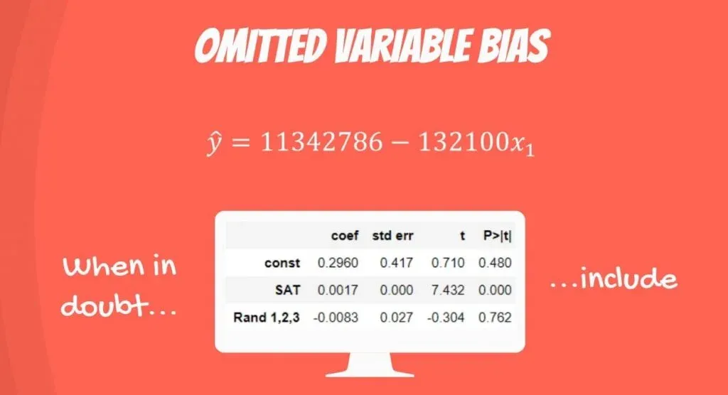
Important: The incorrect exclusion of a variable, like in this case, leads to biased and counterintuitive estimates that are toxic to our regression analysis. An incorrect inclusion of a variable, as we saw in our adjusted R-squared tutorial, leads to inefficient estimates. They don’t bias the regression, so you can immediately drop them. When in doubt, just include the variables and try your luck.

Dealing with Omitted Variable Bias

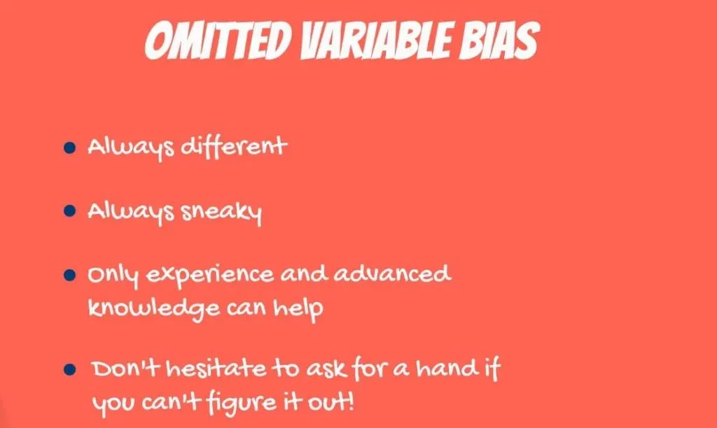
What’s the bottom line? Omitted variable bias is a pain in the neck.

• It is always different
• Always sneaky
• Only experience and advanced knowledge on the subject can help.
• Always check for it and if you can’t think of anything, ask a colleague for assistance!

OLS Assumption 3: Normality and Homoscedasticity

So far, we’ve seen assumptions one and two. Here’s the third one. It comprises three parts:

• normality
• zero mean
• and homoscedasticity

of the error term.

Normality

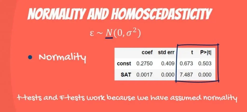
The first one is easy. We assume the error term is normally distributed.

Normal distribution is not required for creating the regression but for making inferences. All regression tables are full of t-statistics and F-statistics.

These things work because we assume normality of the error term. What should we do if the error term is not normally distributed? The central limit theorem will do the job. For large samples, the central limit theorem applies for the error terms too. Therefore, we can consider normality as a given for us.

Zero Mean

What about a zero mean of error terms? Well, if the mean is not expected to be zero, then the line is not the best fitting one. However, having an intercept solves that problem, so in real-life it is unusual to violate this part of the assumption.

Homoscedasticity

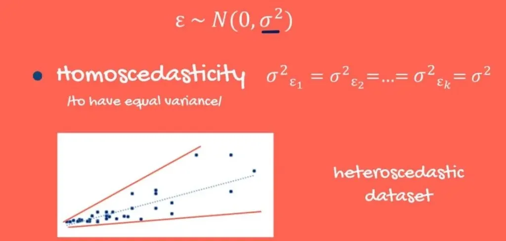
Homoscedasticity means to have equal variance. So, the error terms should have equal variance one with the other.

What if there was a pattern in the variance?

Well, an example of a dataset, where errors have a different variance, looks like this:

It starts close to the regression line and goes further away. This would imply that, for smaller values of the independent and dependent variables, we would have a better prediction than for bigger values. And as you might have guessed, we really don’t like this uncertainty.

A Real-Life Example

Most examples related to income are heteroscedastic with varying variance. If a person is poor, he or she spends a constant amount of money on food, entertainment, clothes, etc. The wealthier an individual is, the higher the variability of his expenditure.

For instance, a poor person may be forced to eat eggs or potatoes every day. Both meals cost a similar amount of money. A wealthy person, however, may go to a fancy gourmet restaurant, where truffles are served with expensive champagne, one day. And on the next day, he might stay home and boil eggs. The variability of his spending habits is tremendous; therefore, we expect heteroscedasticity.

Preventing Heteroscedasticity

There is a way to circumvent heteroscedasticity.

1. First, we should check for omitted variable bias – that’s always an idea.
2. After that, we can look for outliers and try to remove them.
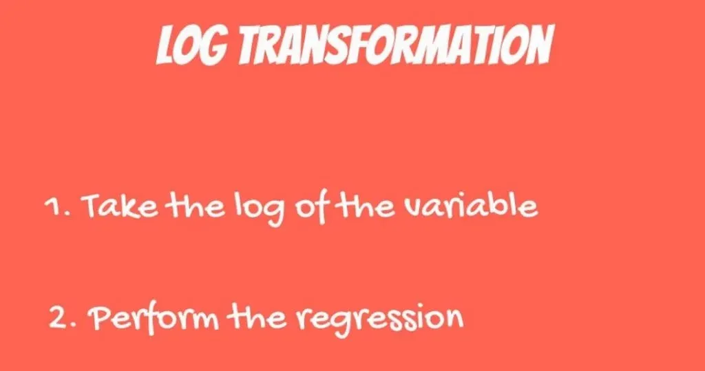
3. Finally, we shouldn’t forget about a statistician’s best friend – the log- transformation.

Naturally, log stands for a logarithm. You can change the scale of the graph to a log scale. For each observation in the dependent variable, calculate its natural log and then create a regression between the log of y and the independent Xs.

Conversely, you can take the independent X that is causing you trouble and do the same.

The Log-Transformation

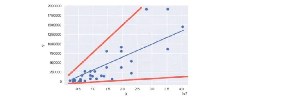
Let’s see an example. Below, you can see a scatter plot that represents a high level of heteroscedasticity.

On the left-hand side of the chart, the variance of the error is small. Whereas, on the right, it is high.

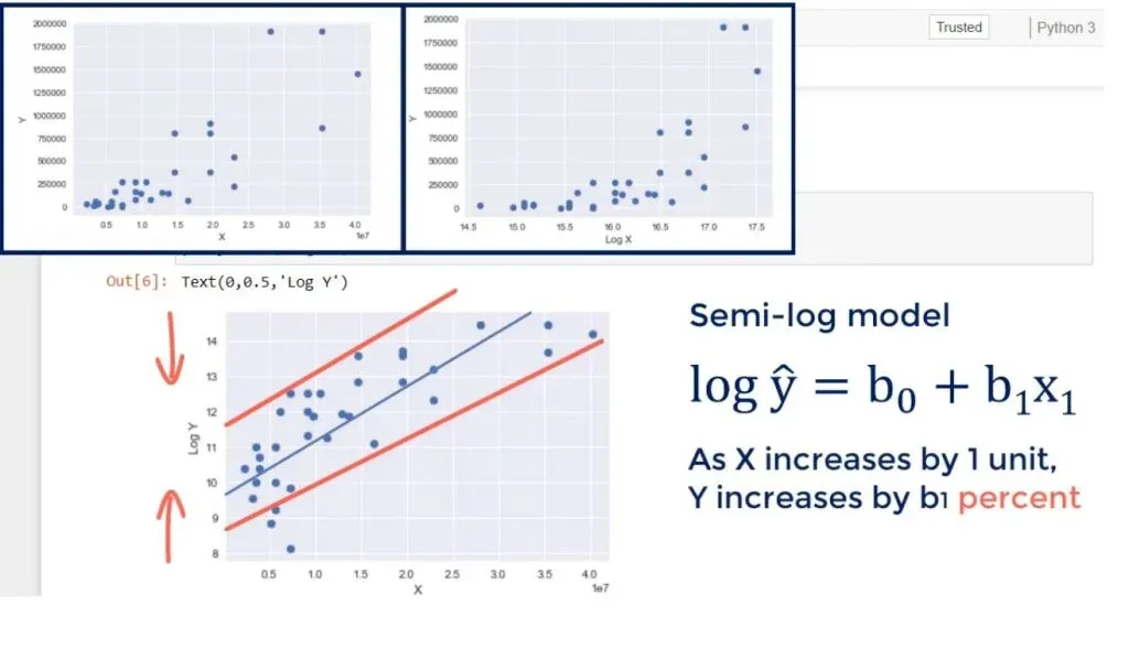
Here’s the model: as X increases by 1 unit, Y grows by b₁ units.

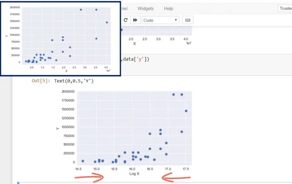
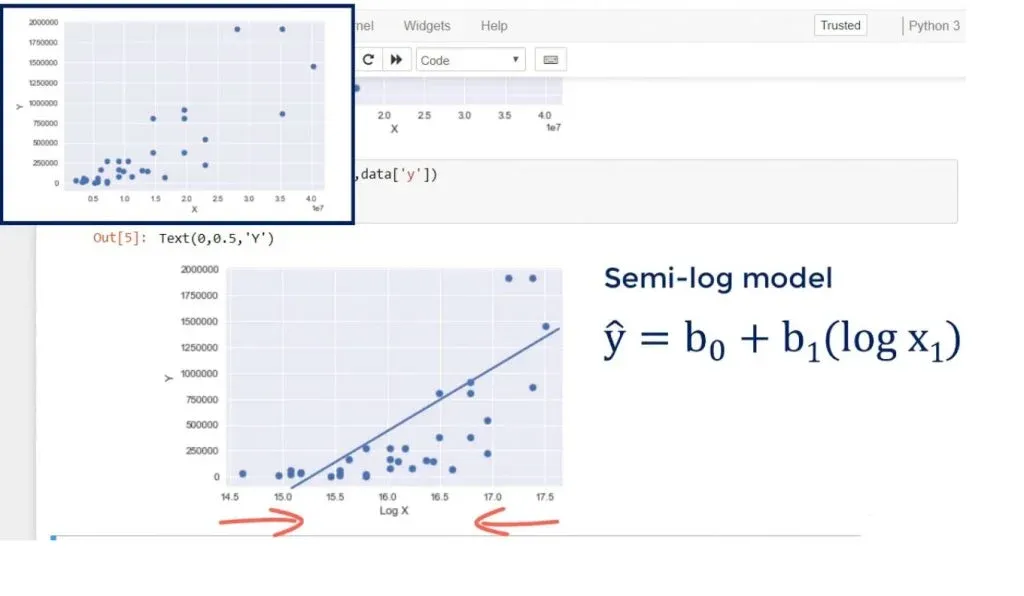
Let’s transform the x variable to a new variable, called log of x, and plot the data. This is the new result.

Changing the scale of x would reduce the width of the graph. You can see how the points came closer to each other from left to right. The new model is called a semi-log model.

Transforming the Y Scale

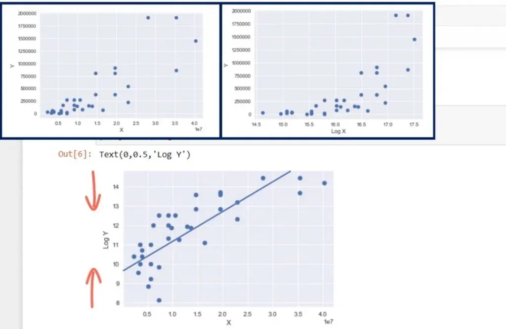
What if we transformed the y scale, instead? Analogically to what happened previously, we would expect the height of the graph to be reduced.

The result is the following:

This looks like good linear regression material. The heteroscedasticity we observed earlier is almost gone. This new model is also called a semi-log model. Its meaning is, as X increases by 1 unit, Y changes by b₁ percent! This is a very common transformation.

The Log-Log Model

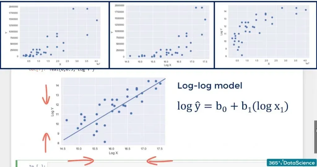
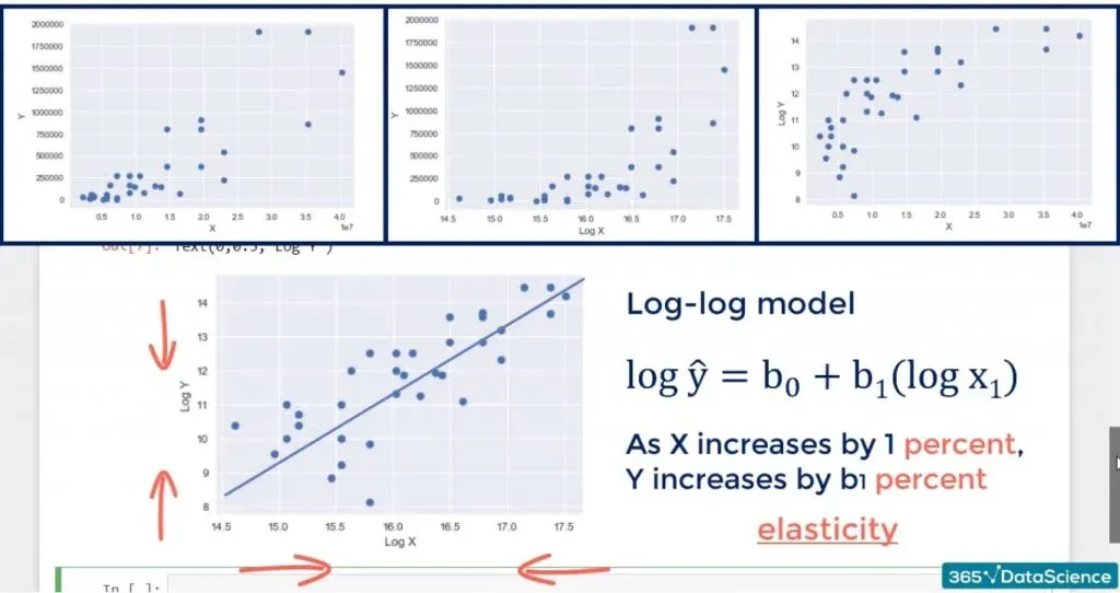
Sometimes, we want or need to change both scales to log. The result is a log-log model. We shrink the graph in height and in width.

You can see the result in the picture below.

The improvement is noticeable, but not game-changing. However, we may be sure the assumption is not violated. The interpretation is, for each percentage point change in x, y changes by b₁ percentage points. If you’ve done economics, you would recognize such a relationship is known as elasticity.

OLS Assumption 4: No Autocorrelation

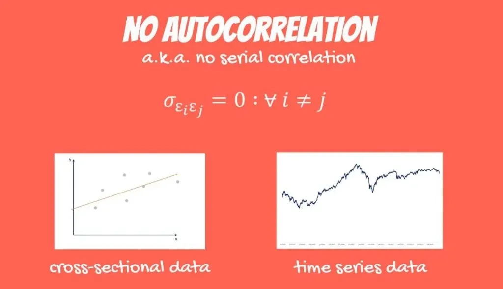
The penultimate OLS assumption is the no autocorrelation assumption. It is also known as no serial correlation. Unfortunately, it cannot be relaxed.

Mathematically, it looks like this: errors are assumed to be uncorrelated.

Where can we observe serial correlation between errors? It is highly unlikely to find it in data taken at one moment of time, known as cross-sectional data. However, it is very common in time series data.

Stock Prices

Think about stock prices – every day, you have a new quote for the same stock. These new numbers you see have the same underlying asset. We won’t go too much into the finance. But basically, we want them to be random or predicted by macro factors, such as GDP, tax rate, political events, and so on.

Unfortunately, it is common in underdeveloped markets to see patterns in the stock prices.

The Day-of-the-Week-Effect

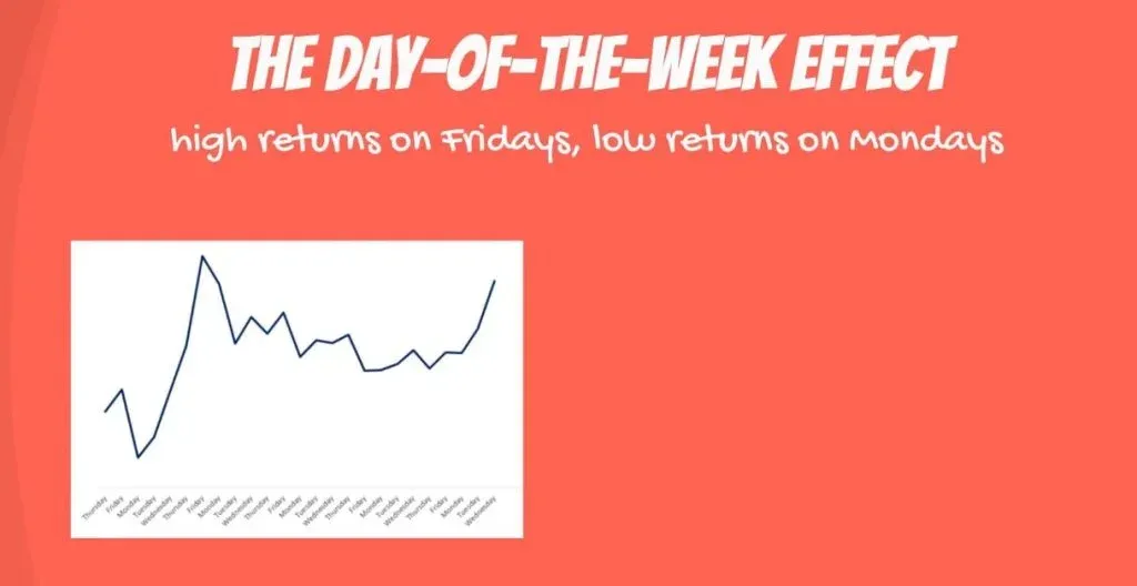
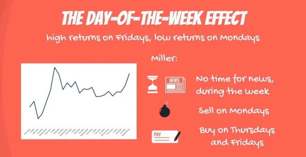
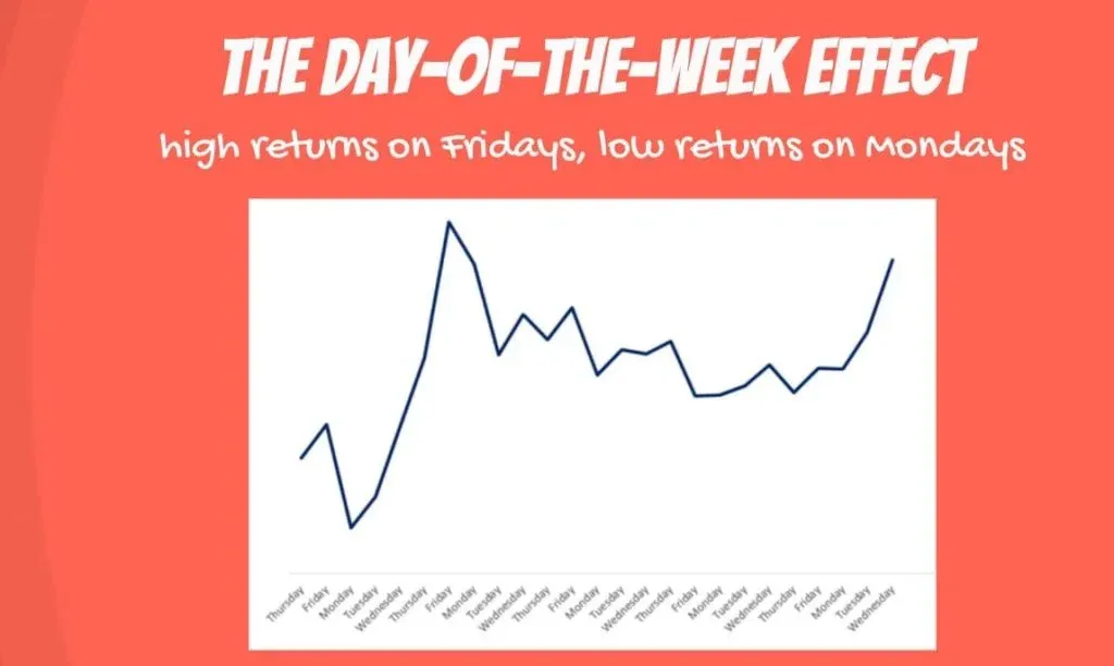
There is a well-known phenomenon, called the day-of-the-week effect. It consists in disproportionately high returns on Fridays and low returns on Mondays. There is no consensus on the true nature of the day of the week effect.

One possible explanation, proposed by Nobel prize winner Merton Miller, is that investors don’t have time to read all the news immediately. So, they do it over the weekend. The first day to respond to negative information is on Mondays. Then, during the week, their advisors give them new positive information, and they start buying on Thursdays and Fridays.

Another famous explanation is given by the distinguished financier Kenneth French, who suggested firms delay bad news for the weekends, so markets react on Mondays.

Correlation of the Errors

Whatever the reason, there is a correlation of the errors when building regressions about stock prices. The first observation, the sixth, the eleventh, and every fifth onwards would be Mondays. The fifth, tenth, and so on would be Fridays. Errors on Mondays would be biased downwards, and errors for Fridays would be biased upwards.

The mathematics of the linear regression does not consider this. It assumes errors should be randomly spread around the regression line.

How to Detect Autocorrelation

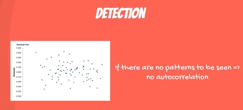
A common way is to plot all the residuals on a graph and look for patterns. If you can’t find any, you’re safe.

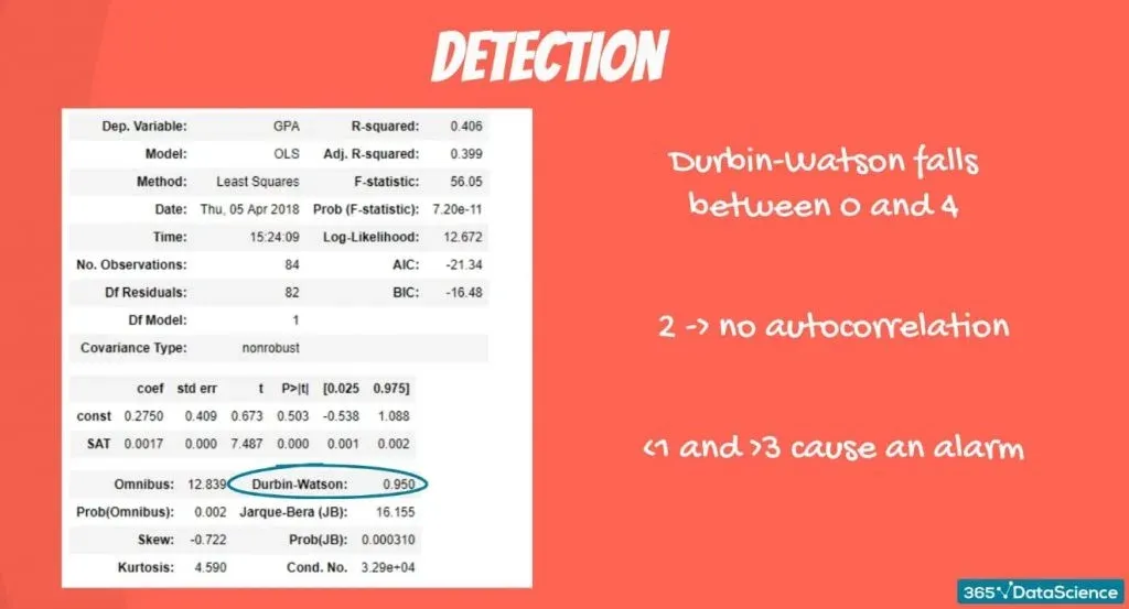
Another is the Durbin-Watson test which you have in the summary for the table provided by ‘statsmodels’. Generally, its value falls between 0 and 4. 2 indicates no autocorrelation. Whereas, values below 1 and above 3 are a cause for alarm.

The Remedy

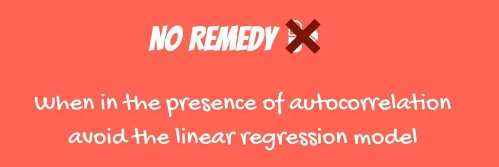
But, what’s the remedy you may ask? Unfortunately, there is no remedy. As we mentioned before, we cannot relax this OLS assumption. The only thing we can do is avoid using a linear regression in such a setting.

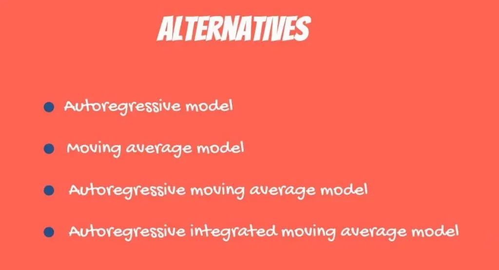
There are other types of regressions that deal with time series data. It is possible to use an autoregressive model, a moving average model, or even an autoregressive moving average model. There’s also an autoregressive integrated moving average model.

Make your choice as you will, but don’t use the linear regression model when error terms are autocorrelated.

OLS Assumption 5: No Multicollinearity

The last OLS assumption is no multicollinearity.

We observe multicollinearity when two or more variables have a high correlation.

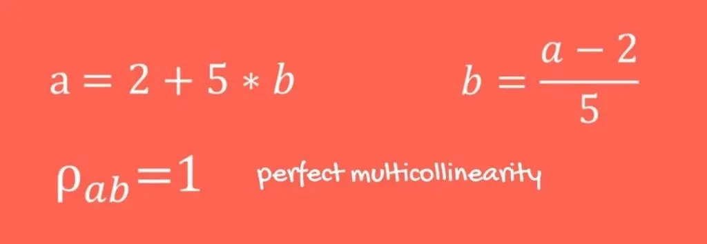
Let’s exemplify this point with an equation.

a and b are two variables with an exact linear combination. a can be represented using b, and b can be represented using a. In a model containing a and b, we would have perfect multicollinearity.

This imposes a big problem to our regression model as the coefficients will be wrongly estimated. The reasoning is that, if a can be represented using b, there is no point using both. We can just keep one of them.

Providing a Case in Point

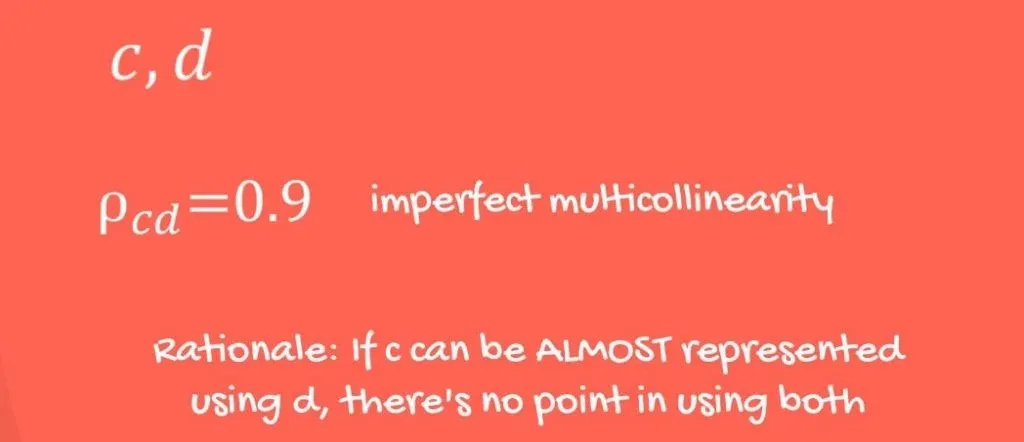
Another example would be two variables c and d with a correlation of 90%. If we had a regression model using c and d, we would also have multicollinearity, although not perfect. Here, the assumption is still violated and poses a problem to our model.

A Real-Life Example

Usually, real-life examples are helpful, so let’s provide one.

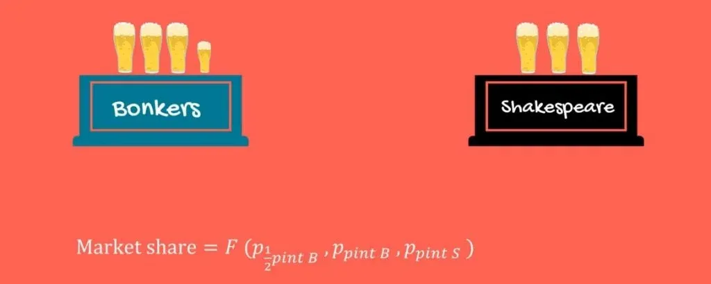
There are two bars in the neighborhood – Bonkers and the Shakespeare bar. We want to predict the market share of Bonkers. Most people living in the neighborhood drink only beer in the bars. So, a good approximation would be a model with three variables: the price of half a pint of beer at Bonkers, the price of a pint of beer at Bonkers, and the price of a pint of beer at Shakespeare’s.

This should make sense. If one bar raises prices, people would simply switch bars.

So, the price in one bar is a predictor of the market share of the other bar.

The Problem

Well, what could be the problem? Half a pint of beer at Bonkers costs around 1 dollar, and one pint costs 1.90. Bonkers tries to gain market share by cutting its price to 90 cents. It cannot keep the price of one pint at 1.90, because people would just buy 2 times half a pint for 1 dollar 80 cents. Bonkers management lowers the price of the pint of beer to 1.70.

Running a Regression

Let’s see what happens when we run a regression based on these three variables. Take a look at the p-value for the pint of beer at Bonkers and half a pint at Bonkers. They are insignificant!

This is because the underlying logic behind our model was so rigid! Well, no multicollinearity is an OLS assumption of the calculations behind the regression. The price of half a pint and a full pint at Bonkers definitely move together.

This messed up the calculations of the computer, and it provided us with wrong estimates and wrong p-values.

How to Fix it

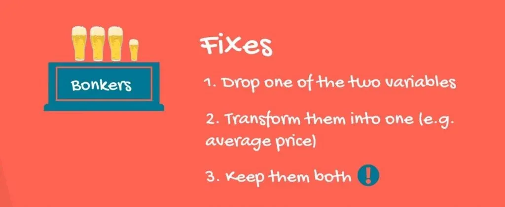
There are three types of fixes:

1. The first one is to drop one of the two variables.
2. The second is to transform them into one variable.
3. The third possibility is tricky. If you are super confident in your skills, you can keep them both, while treating them with extreme caution.

The correct approach depends on the research at hand.

Multicollinearity is a big problem but is also the easiest to notice. Before creating the regression, find the correlation between each two pairs of independent variables. After doing that, you will know if a multicollinearity problem may arise.

Summary of the 5 OLS Assumptions and Their Fixes

Let’s conclude by going over all OLS assumptions one last time.

1. The first OLS assumption is linearity. It basically tells us that a linear regression model is appropriate. There are various fixes when linearity is not present. We can run a non-linear regression or perform a mathematical transformation.
2. The second one is no endogeneity. It means that there should be no relationship between the errors and the independent variables. This is called omitted variable bias and it is not as easy to fix, nor recognize. The best thing you can do is to develop further expertise in the domain or ask someone to help you with fresh eyes.
3. Normality and homoscedasticity are next. Normality suggests that the error term is normally distributed. Homoscedasticity, on the other hand, proposes that the error terms should have equal variance. The way to circumvent heteroscedasticity consists of the following 3 steps: looking for omitted variable bias, removing outliers, and performing a transformation – usually a log transformation works well.
4. Another OLS assumption is no autocorrelation. Here, the idea is that errors are assumed to be uncorrelated. The twist is that, although you may spot it by plotting residuals on a graph and looking for patterns, you cannot actually fix it. Your only option is to avoid using a linear regression in that case.
5. The last OLS assumption is called no multicollinearity. It means that there shouldn’t be high linear dependence between 2 or more variables. There are 3 common ways to deal with You can drop one of the 2 variables or transform them into one variable. You can also keep both of them, but you should be very careful.

The Next Challenge: Representing Categorical Data via Regressions

So, if you understood the whole article, you may be thinking that anything related to linear regressions is a piece of cake. Yes, and no. There are some peculiarities.

Like: how about representing categorical data via regressions? How can it be done? Find the answers to all of those questions in the following tutorial.

***

Interested in learning more? You can take your skills from good to great with our statistics course!

Try statistics course for free

Next Tutorial: How to Include Dummy Variables into a Regression