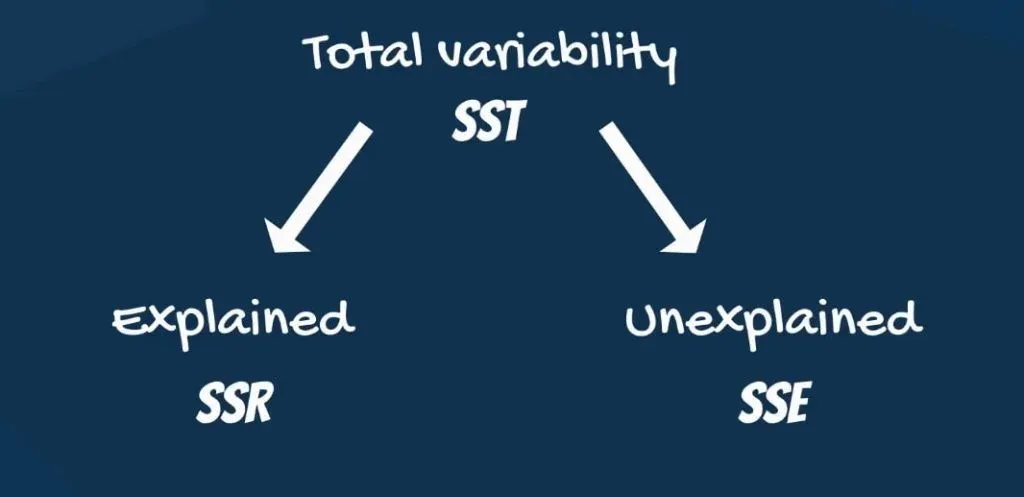
If you are looking for a widely-used measure that describes how powerful a regression is, the R-squared will be your cup of tea. A prerequisite to understanding the math behind the R-squared is the decomposition of the total variability of the observed data into explained and unexplained.
A key highlight from that decomposition is that the smaller the regression error, the better the regression.
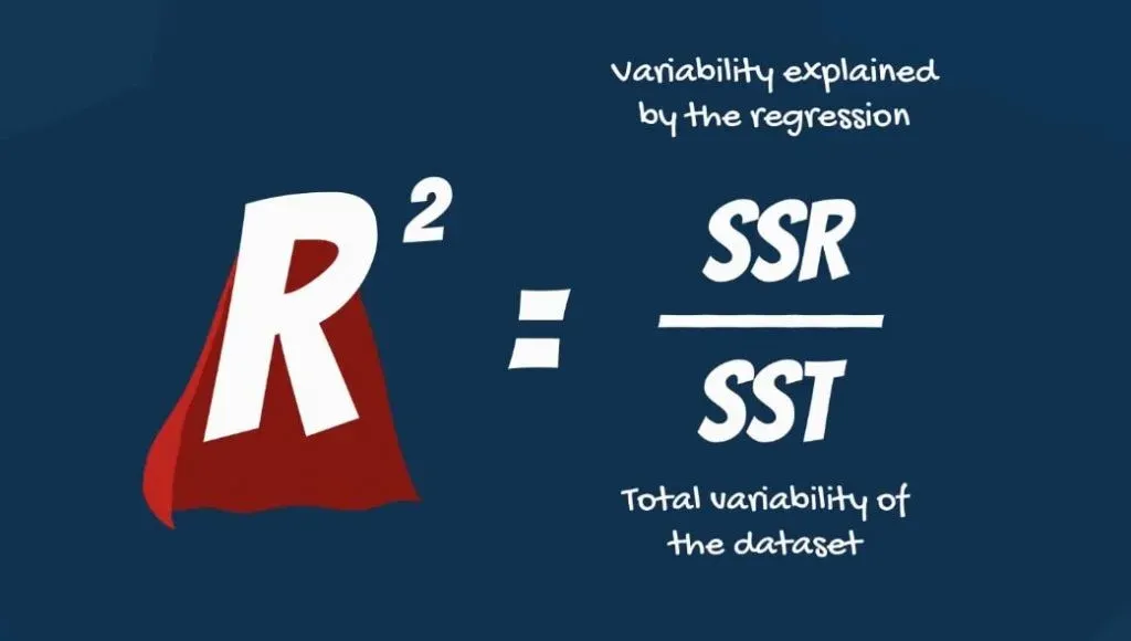
Now, it’s time to introduce you to the R-squared. The R-squared is an intuitive and practical tool, when in the right hands. It is equal to variability explained by the regression, divided by total variability.
What Exactly is the R-squared?
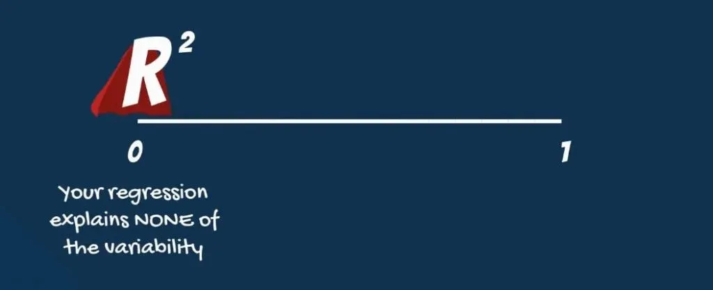
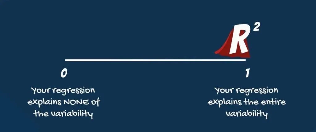
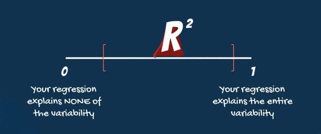
It is a relative measure and takes values ranging from 0 to 1. An R-squared of zero means our regression line explains none of the variability of the data.
An R-squared of 1 would mean our model explains the entire variability of the data.
Unfortunately, regressions explaining the entire variability are rare. What we usually observe are values ranging from 0.2 to 0.9.
What's the Best Value for an R-squared?
The immediate question you may be asking: “What is a good R-squared? When do I know, for sure, that my regression is good enough?”
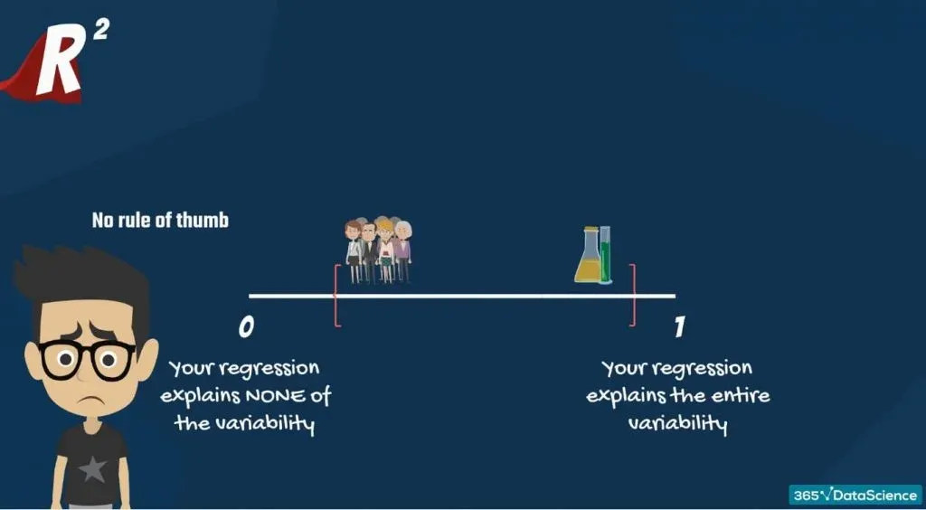
Unfortunately, there is no definite answer to that.
In fields such as physics and chemistry, scientists are usually looking for regressions with R-squared between 0.7 and 0.99. However, in social sciences, such as economics, finance, and psychology the situation is different. There, an R-squared of 0.2, or 20% of the variability explained by the model, would be fantastic.
It depends on the complexity of the topic and how many variables are believed to be in play.
Dealing with Multiple Variables
Take your income, for example. It may depend on your household income (including your parents and spouse), your education, years of experience, country you are living in, and languages you speak. However, this may still account for less than 50% of the variability of income.
Your salary is a very complex issue. But you probably know that.
SAT-GPA Example
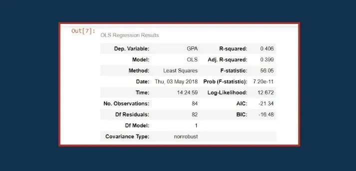
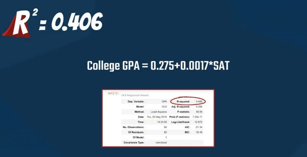
Let’s check out an SAT-GPA example. We have used it in a previous tutorial so if you want to keep track of what we are talking about, make sure you check it out. If you don’t want to, here’s the regression summary:
The SAT score is one of the better determinants of intellectual capacity and capability. The truth is that our regression had an R-squared of 0.406, as you can see in the picture below.
In other words, SAT scores explain 41% of the variability of the college grades for our sample.
Other Factors
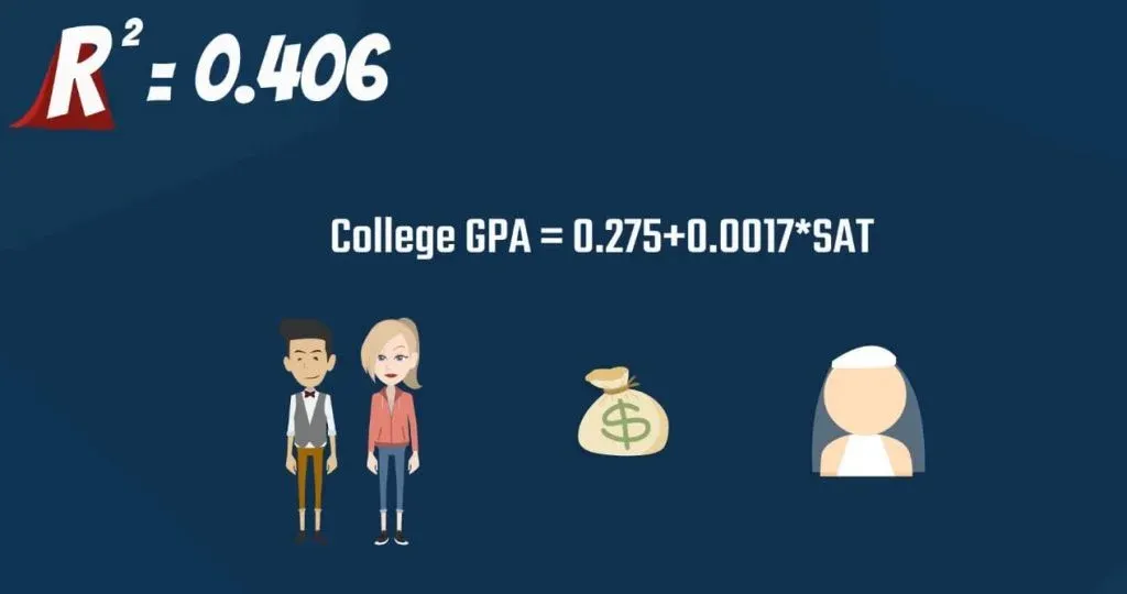
An R-squared of 41% is neither good nor bad. But since it is far away from 90%, we may conclude we are missing some important information. Other determinants must be considered. Variables such as gender, income, and marital status could help us understand the full picture a little better.
Now, you probably feel ready to move on. However, you should remember one thing.
Don’t jump into regressing so easily. Critical thinking is crucial. Before agreeing that a factor is significant, you should try to understand why. So, let’s quickly justify that claim.
Gender
First, women are more likely to outperform men in high school.
But then in higher education, more men enter academia.
There are many biases in place here. Without telling you if female or male candidates are better, scientific research shows that a gender gap exists in education. Gender is an important input for any regression on the topic.
Income
The second factor we pointed out is income. If your household income is low, you are more likely to get a part-time job.
Thus, you’ll have less time for studying and probably get lower grades.
If you’ve ever been to college, you will surely remember a friend who underperformed because of this reason.
Children
Third, if you get married and have a child, you’ll definitely have a lower attendance.
Contrary to what most students think when in college, attendance is a significant factor for your GPA. You may think your time is better spent when skipping a lecture, but your GPA begs to differ.
When to Include More Factors?
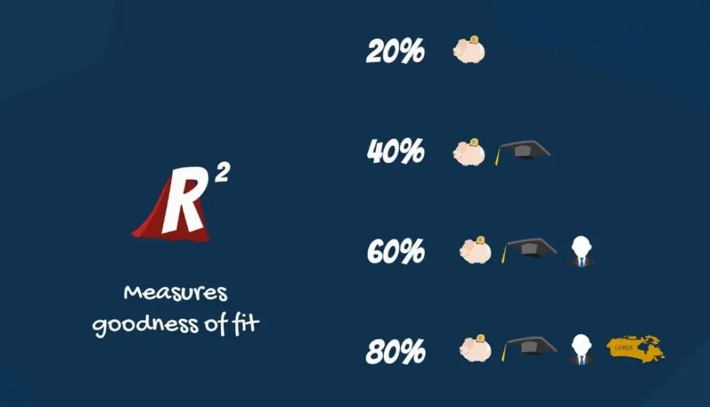
After these clarifications, let’s find the bottom line. The R-squared measures the goodness of fit of our model. The more factors we include in our regression, the higher the R-squared.
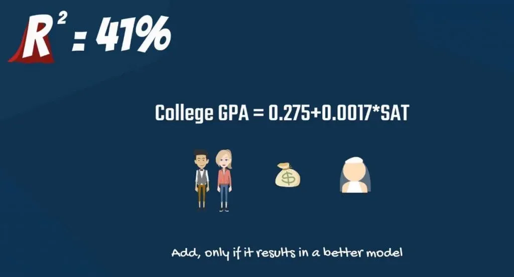
So, should we include gender and income in our regression? If this is in line with our research, and their inclusion results in a better model, we should do that.
The Adjusted R-squared
The R-squared seems quite useful, doesn’t it? However, it is not perfect. To be more precise, we’ll have to refine it. Its new version will be called the adjusted R-squared.
What it Adjusts for
Let’s consider the following two statements:
- The R-squared measures how much of the total variability is explained by our model.
- Multiple regressions are always better than simple ones. This is because with each additional variable that you add, the explanatory power may only increase or stay the same.
Well, the adjusted R-squared considers exactly that. It measures how much of the total variability our model explains, considering the number of variables.
The adjusted R-squared is always smaller than the R-squared, as it penalizes excessive use of variables.
Multiple Regressions
Let’s create our first multiple regression to explain this point.
First, we’ll import all the relevant libraries.
This is what we need to code:
import numpy as np
import pandas as pd
import matplotlib.pyplot as plt
import statsmodels.api as sm
import seaborn
seaborn.set()
We can load the data from the file ‘1.02. Multiple linear regression.csv’. You can download it from the following link. The way to load it is the following:
data = pd.read_csv(‘1.02. Multiple linear regression.csv’)An Additional Variable
Let’s type ‘data’ and run the code.
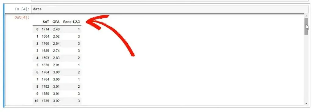
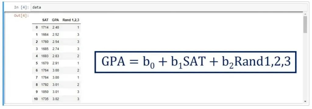
As you can see from the picture above, we have data about the SAT and GPA results of students. However, there is one additional variable, called Rand 1,2,3. We’ve generated a variable that assigns 1, 2, or 3, randomly to each student. We are 100% sure that this variable cannot predict college GPA.
So, this is our model: college GPA is equal to b0+ b1 * SAT score +b2 * the random variable.
Now, let’s write ‘data.describe()’ and see the descriptive statistics.
Creating the Regression
In our case, y is GPA and there are 2 explanatory variables – SAT and Random 1,2,3.
What we can do is declare x1 as a data frame, containing both series. So, the code should look like this:
y = data[‘GPA’]
x1 = data[[‘SAT’, ‘Rand 1,2,3’]]
we must fit the regression:
x = sm.add_constant(x1)
results = sm.OLS(y,x).fit()
After that, we can check out the regression tables using the appropriate method
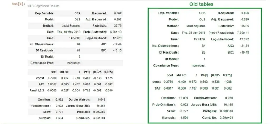
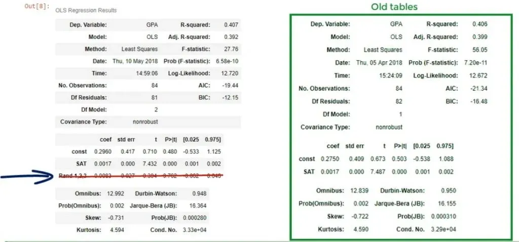
results.summary()You can see the ones from the previously linked tutorial in the box on the right. Keep in mind, that we only have 1 variable there.
The New R-squared
We notice that the new R-squared is 0.407, so it seems as we have increased the explanatory power of the model. But then our enthusiasm is dampened by the adjusted R-squared of 0.392. 
We were penalized for adding an additional variable that had no strong explanatory power. We have added information but have lost value.
Important: The point is that you should cherry-pick your data and exclude useless information.
However, one would assume regression analysis is smarter than that. Adding an impractical variable should be pointed out by the model in some way.
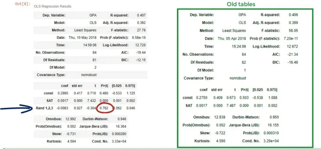
Well, that’s true. Let’s take a look at the coefficients table. We have determined a coefficient for the Rand 1,2,3 variable, but its P-value is 0.762!
The Null Hypothesis
The null hypothesis of the test is that β = 0. We cannot reject the null hypothesis at the 76% significance level!
This is an incredibly high P-value.
Important: For a coefficient to be statistically significant, we usually want a P-value of less than 0.05.
Our conclusion is that the variable Rand 1,2,3 not only worsens the explanatory power of the model, reflected by a lower adjusted R-squared but is also insignificant. Therefore, it should be dropped altogether.
Dropping Useless Variables
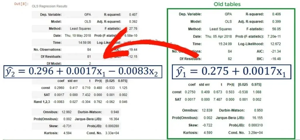
Dropping useless variables is important. You can see the original model changed from:
ŷ = 0.275 + 0.0017* x1
to
ŷ = 0.296+ 0.0017* x1- 0.0083 * x2
The choice of the third variable affected the intercept. Whenever you have one variable that is ruining the model, you should not use this model altogether. This is because the bias of this variable is reflected in the coefficients of the other variables. The correct approach is to remove it from the regression and run a new one, omitting the problematic predictor. 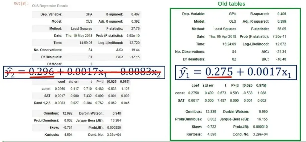
Simplicity
There is one more consideration concerning the removal of variables from a model. We can add 100 different variables to a model and probably the predictive power of the model will be outstanding. However, this strategy makes regression analysis futile. We are trying to use a few independent variables that approximately predict the result. The trade-off is complex, but simplicity is better rewarded than higher explanatory power.
How to Compare Regression Models?
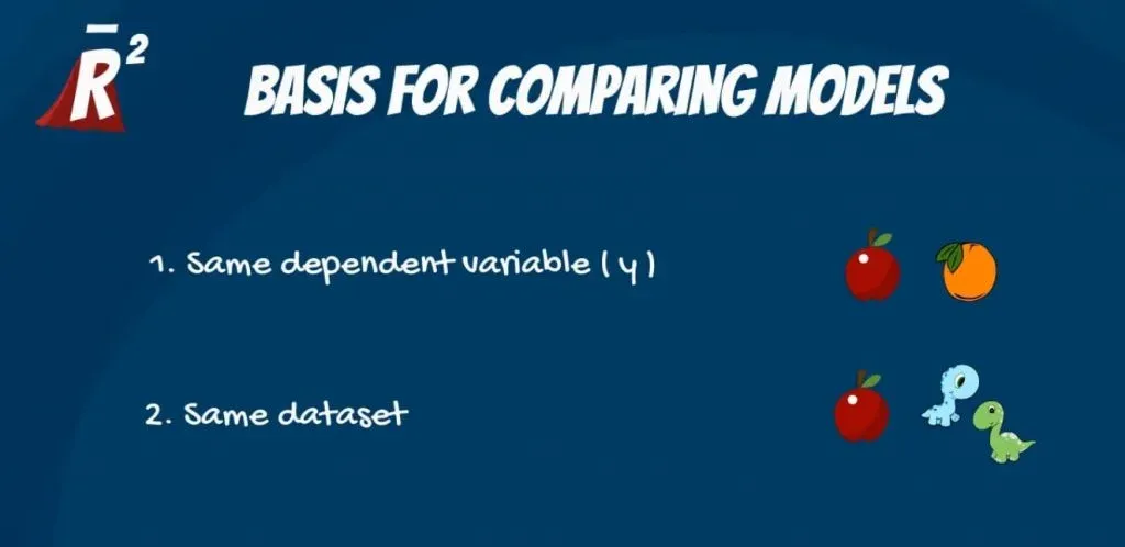
Finally, the adjusted R-squared is the basis for comparing regression models. Once again, it only makes sense to compare two models considering the same dependent variable and using the same dataset. If we compare two models that are about two different dependent variables, we will be making an apples-to-oranges comparison. If we use different datasets, it is an apples-to-dinosaurs problem.
As you can see, adjusted R-squared is a step in the right direction, but should not be the only measure trusted. Caution is advised, whereas thorough logic and diligence are mandatory.
What We’ve Learned
To sum up, the R-squared basically tells us how much of our data’s variability is explained by the regression line. The best value for an R-squared depends on the particular case. When we feel like we are missing important information, we can simply add more factors. This is where the adjusted R-squared comes into play. It measures the variability of our model but it also considers the number of variables. Therefore, it is always smaller than the R-squared. Moreover, the adjusted R-squared is the basis for comparing regression models.
After reading this, you probably feel like you are ready to dive deeper into the field of linear regressions. Maybe you are keen to find out how to estimate a linear regression equation. Or maybe you want to know what to consider before performing regression analysis.
Either way, exploring the world of the Ordinary Least Squares assumptions will be right up your street.
***
Interested in learning more? You can take your skills from good to great with our statistics tutorials and Statistics course.
Next Tutorial: Exploring the OLS Assumptions

