If you want to expand your knowledge in statistics, understanding how the Central Limit Theorem works, will be right up your street.
Before we start, you can also watch our video on the topic - just press "play" below or scroll down if you prefer reading.
First, let’s introduce a concept – a sampling distribution.
Sampling Distribution
Say you have the population of used cars in a car shop.
We want to analyze the car prices and be able to make some predictions on them. Population parameters which may be of interest are:
- mean car price
- standard deviation of prices
- covariance
- and so on.
Normally, in statistics, we would not have data on the whole population, but rather just a sample.
Drawing a Sample
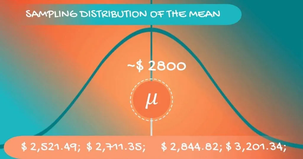
The mean is $2,617.23.
Now, a problem arises from the following fact. If we take another sample, we may get a completely different mean - $3,201.34.
Then a third with a mean of $2,844.33.
As you can see, the sample mean depends on the incumbents of the sample itself. So, taking a single value is definitely suboptimal.
Drawing Many Samples
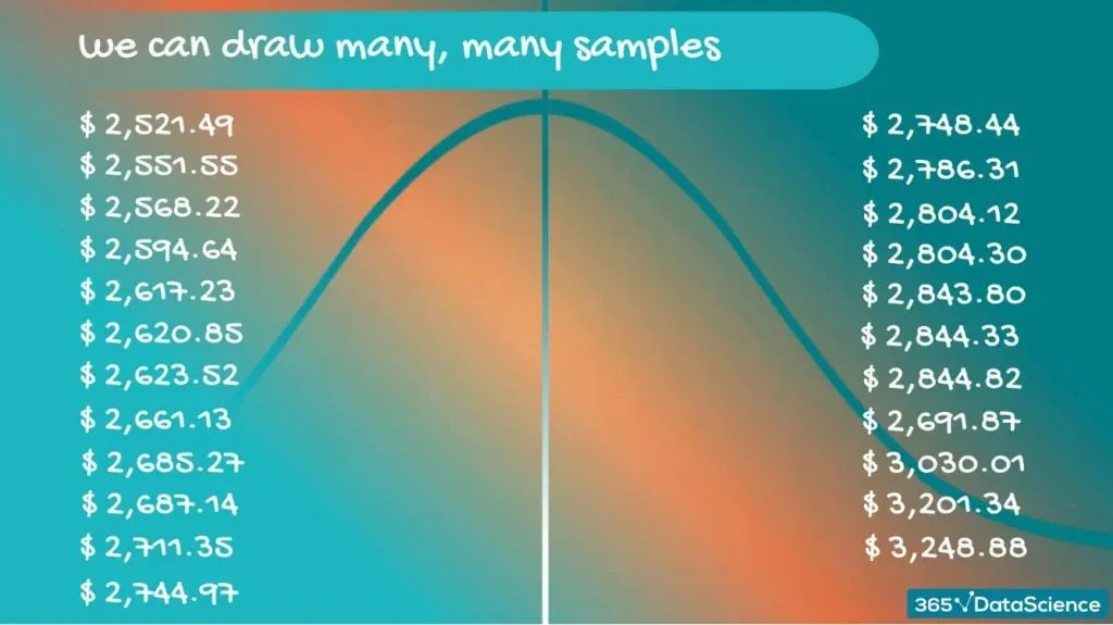
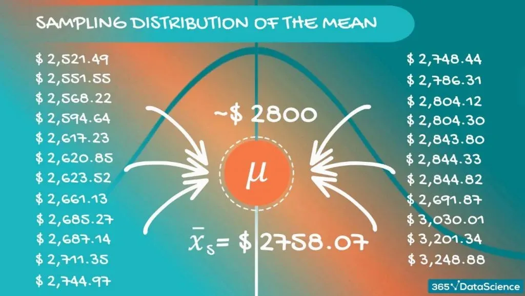
What we can do is draw many, many samples and create a new dataset, comprised of sample means.
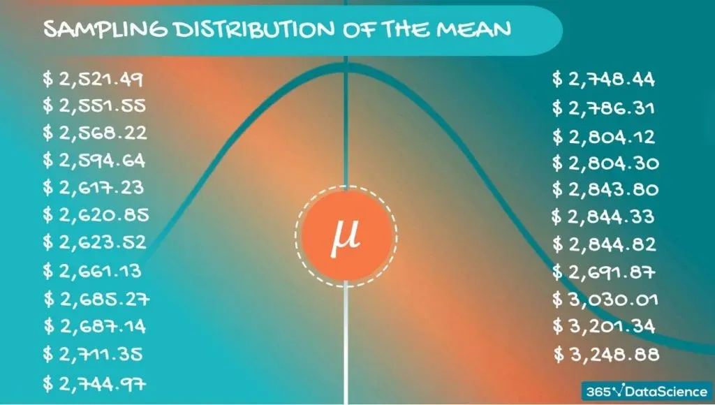
These values are distributed in some way, so we have a distribution. When we are referring to a distribution formed by samples, we use the term - a sampling distribution. For our case, we can be even more precise – we are dealing with a sampling distribution of the mean.
The Population Mean
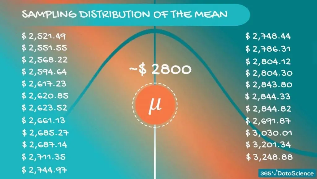
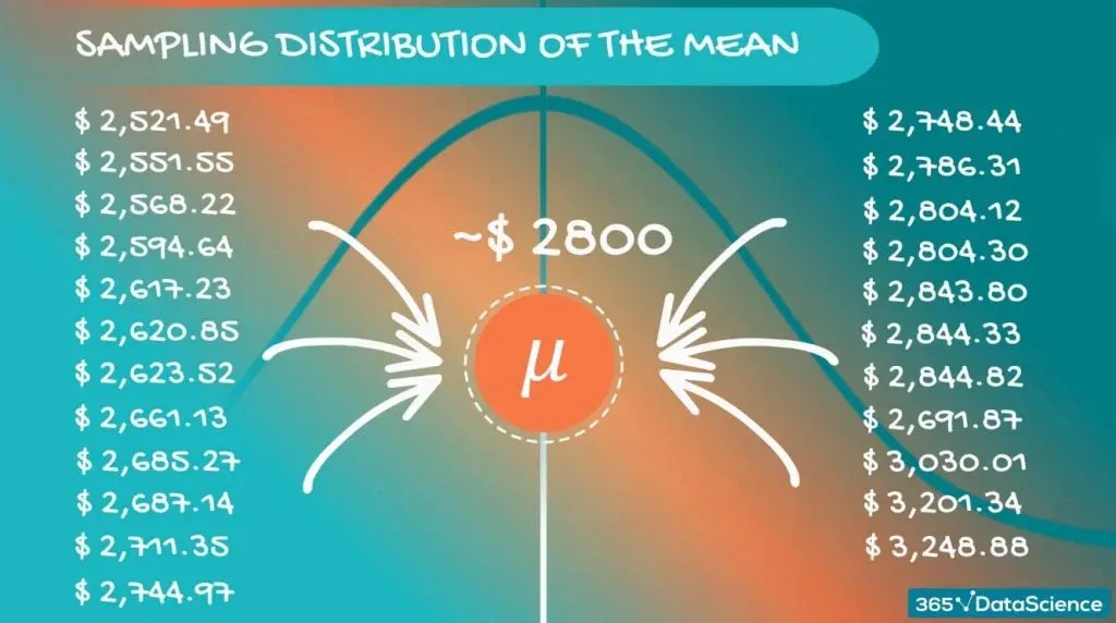
Now, if we inspect these values closely, we will realize that they are different. However, they are concentrated around a certain value. For our case - somewhere around $2,800.
Each of these sample means is nothing but an approximation of the population mean. The value they revolve around is actually the population mean itself. Most probably, none of them are the population mean, but taken together, they give a really good idea.
In fact, if we take the average of those sample means, we expect to get a very precise approximation of the population mean.
Visualizing the Distribution of the Sampling Means
Here’s a plot of the distribution of the car prices.
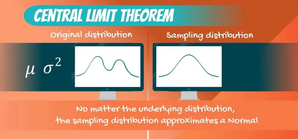
We know that this is not a normal distribution. It has a right skew and that’s about all we can see.
Here’s the big revelation.
It turns out that if we visualize the distribution of the sampling means, we get something else. Something useful.
A normal distribution.
And that’s what the Central Limit Theorem states.
The Central Limit Theorem
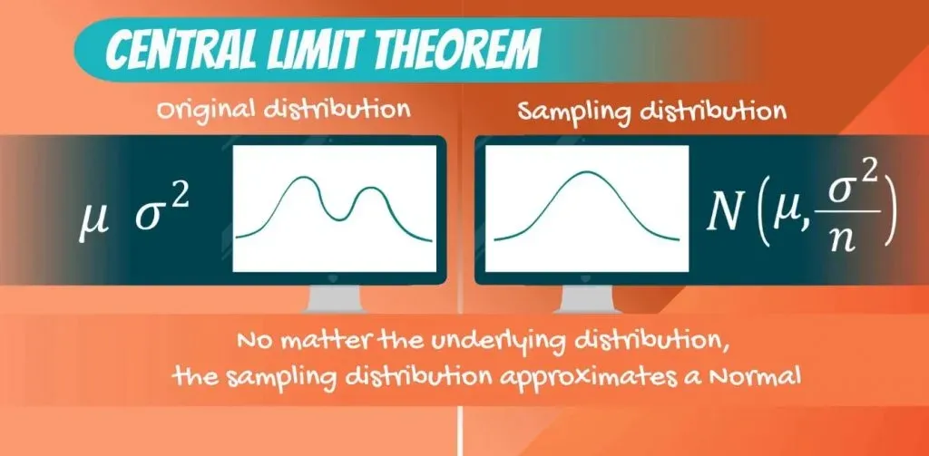
The sampling distribution of the mean will approximate a normal distribution. No matter the distribution of the population - Binomial, Uniform, Exponential or another one.
Not only that, but its mean is the same as the population mean.
That’s something we already noticed.
The Variance
What about the variance?
Well, it depends on the size of the samples we draw but it is quite elegant. It is the population variance divided by the sample size.
Since the sample size is in the denominator, the bigger the sample size, the lower the variance. Or in other words – the closer the approximation we get. So, if you are able to draw bigger samples, your statistical results will be more accurate. Usually for the Central Limit Theorem to apply, we need a sample size of at least 30 observations.
Why the Central Limit Theorem is Important
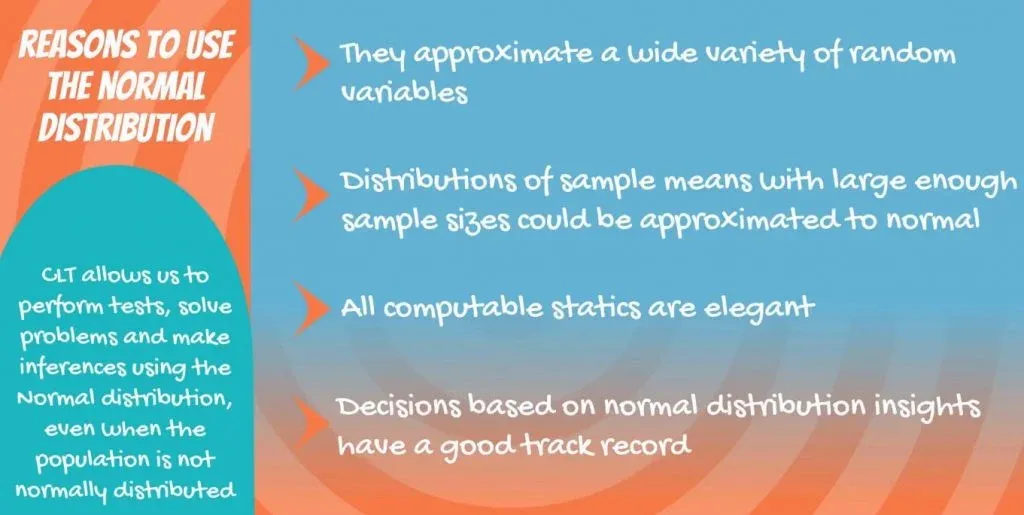
The Central Limit Theorem allows us to perform tests, solve problems and make inferences using the normal distribution even when the population is not normally distributed.
Even more so, the normal distribution has elegant statistics and unmatched applicability in calculating confidence intervals and performing tests. So, if you’re looking to streamline your statistical calculations, our range of advanced calculators can help you quickly perform various analyses, including those dealing with Confidence Intervals.
The discovery and proof of the theorem revolutionized statistics as a field and we will be relying on it a lot in the subsequent tutorials.
Standard error
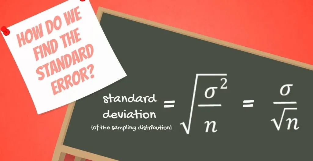
Now, there is another important notion which spurs from the sampling distribution and is closely related to CLT. The standard error. It is the standard deviation of the distribution formed by the sample means.
In other words – the standard deviation of the sampling distribution.
So how do we find it? We know its variance: sigma squared, divided by n. Therefore, the standard deviation is sigma, divided by the square root of n.
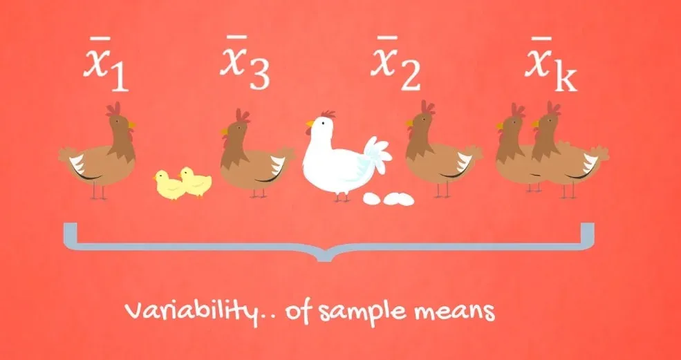
Like a standard deviation, the standard error shows variability. In this case, it is the variability of the means of the different samples we extracted.
You can guess that since the term has its own name, it is widely used and very important.
Why We Need it
Standard error is used for almost all statistical tests. This is because it is a probabilistic measure that shows how well you approximated the true mean.
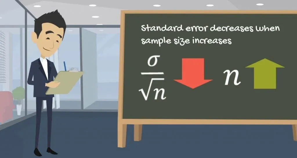
Important: It decreases as the sample size increases! This makes sense, as bigger samples give a better approximation of the population.
What’s Next
To sum up, the Central Limit Theorem states:
No matter the underlying distribution of the data set, the distribution of the sample means would be normal. Moreover, its mean would be equal to the original mean. Its variance, however, would be equal to the original variance divided by the sample size.
Now, if you want to get deeper into the subject of statistics, we have covered just the right concept. Find out how estimators work and what you can use them for, in the linked tutorial.
***
Interested in learning more? You can take your skills from good to great with our statistics course!
Try statistics course for free
Next Tutorial: How to Use Point Estimates and Confidence Intervals


