
When you think of the word data, you probably envision a table with features along the rows and the columns, each cell storing a piece of information. In this article, we dare to go a bit further by stepping beyond those constraints. We will introduce the data cube – a structure for representing data in more than 2 dimensions.
In the upcoming paragraphs, we will build a data cube using an intuitive example, which will help us define its elements and understand what operations can be performed on it. We’ll also touch on the difference between a data cube and a data warehouse, and even take a look at different applications in the field of astronomy.
Table of Contents
- What Is a Data Cube?
- What Are the Data Cube Operations?
- Data Cube vs Data Warehouse
- How to Apply Data Cubes in the Field of Astronomy?
- Data Cube: Next Steps
What is a Data Cube?
According to the formal definition, a data cube refers to a multi-dimensional data structure. That is, data within the data cube is explained by specific dimensional values.
Albeit being called a cube, it doesn’t necessarily live in 3 dimensions, nor does it have equal sides as the name suggests. It can be a two-dimensional (2D) table in the form of a rectangle, a 3D solid in the form of a parallelepiped, or even an impossible-to-visualize 4D structure.
Although not so often, we can also talk about zero- or one-dimensional cubes – the former is represented by a single number, while the latter is constructed by an array of numbers.
What Is an Example of a Data Cube?
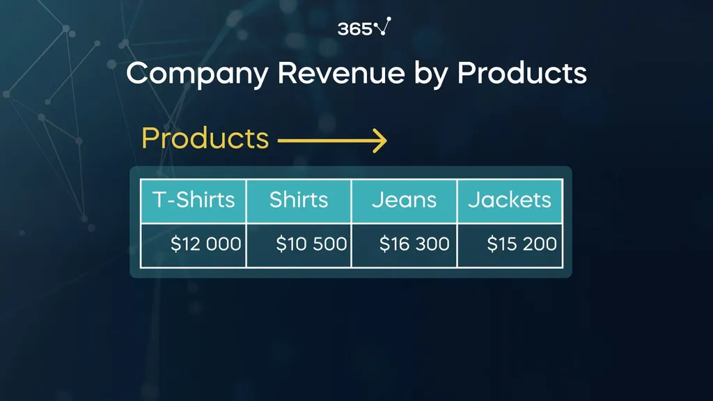
Let’s build our understanding of this concept with the help of a toy data cube example. Consider a retail company based in the United States that offers 4 types of clothing – t-shirts, shirts, jeans, and jackets.
The in-house data engineers have gathered information about last year’s revenue (displayed as a one-dimensional array):
The company, however, has stores in 4 states – California, Hawaii, Indiana, and Michigan. Therefore, the revenue can be split further by products and by states, resulting in a 2D table:
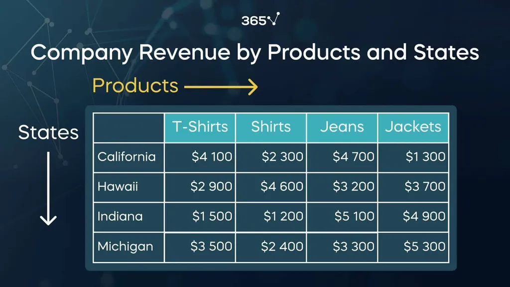
Notice that the sum of the numbers along each of the columns gives the total revenue by product. For example, just the t-shirts alone bring in 12 thousand dollars:
\[\$ 4,100 + \$ 2,900+ \$ 1,500+ \$ 3,500 = \$ 12,000\]
But now, we can sum along the rows as well, such as the annual revenue coming from California:
\[\$ 4,100 + \$ 2,300 + \$ 4,700 + \$ 1,300 = \$ 12,400\]
We can therefore add one more column next to Jackets and call it ‘ALL’. This will represent the annual revenue for each state. Analogously, an additional row (with the same name) can be included below Michigan, storing the annual revenue for each product. These 2 dimensions would meet in a cell in the bottom right corner to show the total annual revenue for the chain retail.
What if we wanted to split this revenue by date? For simplicity, we’ll divide the year into quarters. One way to store the information for all 4 is by constructing separate tables for each:
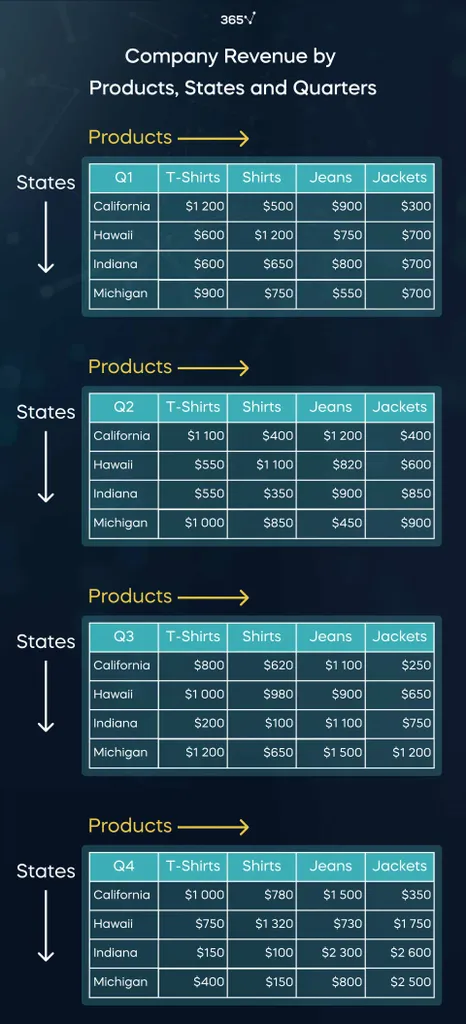
Note that the quarter is specified in the top left cell of each table.
This is not the most elegant solution, is it? As an alternative, we can create a third dimension called ‘Date’ by stacking all 4 tables:
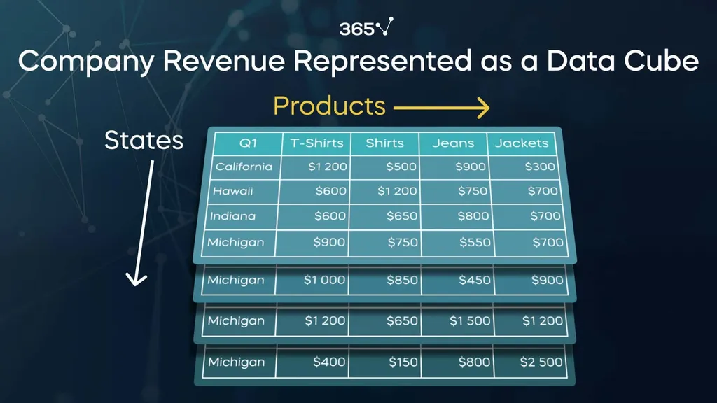
There is now one more dimension that we can sum over. As an example, we’ll calculate the revenue for a full year of t-shirt purchases in Michigan:
\[\$ 900 + \$ 1,000 + \$ 1,200 + \$400 = \$ 3,500\]
Similar to the ‘ALL’ fields for ‘Products’ and ‘States’, we can calculate the total revenue by ‘Date’ as well. In this way, all 3 data cube dimensions will meet in a single data cell, storing the total revenue for a full year.
You are now probably starting to appreciate the functionalities of a data cube. As you can see, it allows us to group data across all dimensions of a cube and retrieve it in an efficient way.
On the other hand, you might be wondering, “What if we added a fourth dimension, say ‘Currency’? How do we visualize this data cube?” The truth is that a cube of more than 3 dimensions cannot be visualized in its entirety. Nevertheless, we can still construct it in an analogous way. We call such multi-dimensional cubes by a special name – hypercubes.
What Are the Elements of a Data Cube?
Now that we’ve laid the foundations, let’s get acquainted with the data cube terminology. Here is a summary of the individual elements, starting from the definition of a data cube itself:
- A data cube is a multi-dimensional data structure.
- A data cube is characterized by its dimensions (e.g., Products, States, Date).
- Each dimension is associated with corresponding attributes (for example, the attributes of the Products dimensions are T-Shirt, Shirt, Jeans and Jackets).
- The dimensions of a cube allow for a concept hierarchy (e.g., the T-shirt attribute in the Products dimension can have its own, such as T-shirt Brands).
- All dimensions connect in order to create a certain fact – the finest part of the cube.
- A fact has a corresponding measure in the data cube. Typically, the fact measure in a data cube for a chain retail business is the revenue (such as the $900 revenue from jeans purchases in Indiana during the second quarter).
What Are the Data Cube Operations?
Data cubes are a very convenient tool whenever one needs to build summaries or extract certain portions of the entire dataset. We will cover the following:
- Rollup – decreases dimensionality by aggregating data along a certain dimension
- Drill-down – increases dimensionality by splitting the data further
- Slicing – decreases dimensionality by choosing a single value from a particular dimension
- Dicing – picks a subset of values from each dimension
- Pivoting – rotates the data cube
Rollup
An important feature of data cubes is aggregating data, which results in dimensionality reduction. We do this by grouping the values across a certain dimension, either by taking their sum, average, standard deviation, or by applying any other aggregate function. This dimensionality reduction procedure is known as a rollup. I like to imagine it as a zooming out on a data cube.
Let’s view it through the lens of our retail example: summing across the ‘Date’ dimension in the 3D cube returns the 2D table displaying only ‘Products’ and ‘States’. If you’re an SQL user, you are well familiar with aggregate functions and know that they are almost always used in combination with the GROUP BY clause.
Drill-down
In contrast, a drill-down of a data cube refers to dimensionality increase. In laymen terms, this would be similar to zooming in on a cube. That is, we split the revenue not only by products, but also by states; or make a split not only by products, but also by product brands.
Slicing
Furthermore, a data cube can also be sliced. What that means is to reduce the number of dimensions by keeping one of them fixed. For example, we can slice our 3D data cube and obtain a two-dimensional one by choosing to study the revenue by products and states only for the first quarter of the year.
Dicing
Rather than extracting a slice from a cube, we can also create a die through dicing. This is done by picking certain values from the dimensions. For example, we can choose to see the revenue from shirts and jeans purchases in Hawaii and Michigan during the first and second quarters.
Pivoting
Lastly, pivoting is when we rotate a data cube, allowing for a dimension to be displayed either along its length, width, or depth.
Data Cube vs Data Warehouse
Data science is anything but lacking in terminology. What often brings confusion among enthusiasts who want to break into this field is how data cubes differ from data warehouses.
What Is a Data Warehouse?
A data warehouse is the place (typically a cloud storage) where a company’s historical data is stored in a structured way, usually in the form of relational databases. They can’t be changed, nor deleted. Rather, we can only retrieve information through aggregation or segmentation and use it for analytical, referential, or reporting purposes. Essentially, it is a company’s single source of data truth.
If you’d like to learn more about data warehouses, check out our video on the topic:
A data cube, on the other hand, refers to the way data is structured, as well as how a company might choose to use the cube technology in a data warehouse. Using the multidimensional approach of OLAP data cubes, for example, is only one way of doing this.
How to Apply Data Cubes in the Field of Astronomy?
Arxiv is an open-source library storing millions of scholarly articles in various science fields. If you search “data cubes” on their website, you will quickly find that papers from the Astronomy section come up surprisingly often. Why is that?
Well, astronomy is a science that relies heavily on images – two-dimensional pixelated objects, with each pixel described by a number (or 3 numbers, if colored). They, however, are often taken at different wavelength bands. A picture taken in the visible range, and one taken in the infra-red spectrum reveal different details about the object of interest.
As a result, the wavelength band could serve as a third dimension in a data cube. The resulting structure is called a hyperspectral data cube. This technology has found its application not only in astronomy, but in almost every field of science – agriculture, medicine, experimental physics, climatology, and many more.
Q&A
Data Cubes: Next Steps
The data cube approach turns out to be a very intuitive and logical way of thinking. It can be an invaluable business intelligence tool, helping data and business analysts to draw meaningful conclusions and create strategies for a company’s growth. Not only that, but it is used widely in other fields of science, mostly in the context of computer vision.
SQL is undoubtedly the language that all data engineers, analysts, and scientists master first. Start your SQL journey now with our comprehensive SQL course. Should you instead want to acquire or enhance your data analysis and visualization skills, then don’t miss our Introduction to Business Analytics course.