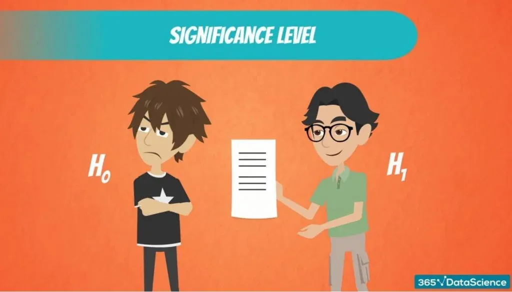
If you want to understand why hypothesis testing works, you should first have an idea about the significance level and the reject region. We assume you already know what a hypothesis is, so let’s jump right into the action.
What Is the Significance Level?
First, we must define the term significance level.
Normally, we aim to reject the null if it is false.
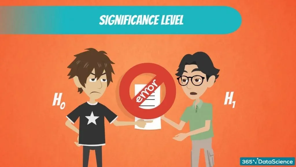
However, as with any test, there is a small chance that we could get it wrong and reject a null hypothesis that is true.
How Is the Significance Level Denoted?
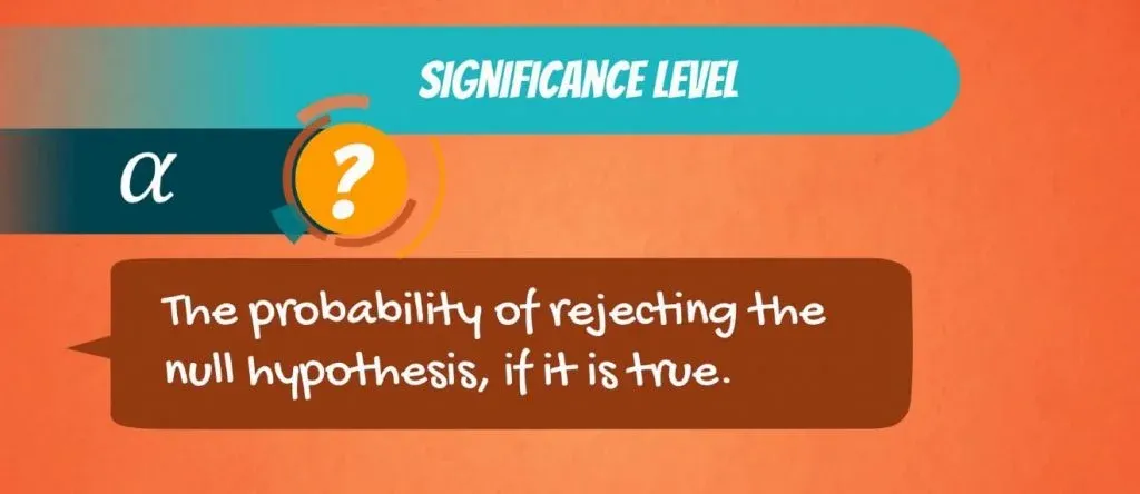
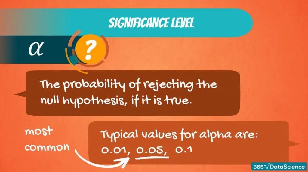
The significance level is denoted by α and is the probability of rejecting the null hypothesis, if it is true.
So, the probability of making this error.
Typical values for α are 0.01, 0.05 and 0.1. It is a value that we select based on the certainty we need. In most cases, the choice of α is determined by the context we are operating in, but 0.05 is the most commonly used value.
A Case in Point
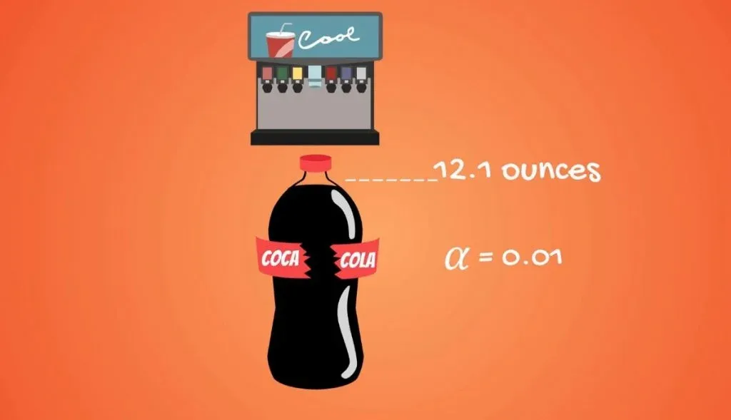
Say, we need to test if a machine is working properly. We would expect the test to make little or no mistakes. As we want to be very precise, we should pick a low significance level such as 0.01.
The famous Coca Cola glass bottle is 12 ounces. If the machine pours 12.1 ounces, some of the liquid would be spilled, and the label would be damaged as well. So, in certain situations, we need to be as accurate as possible.
Higher Degree of Error
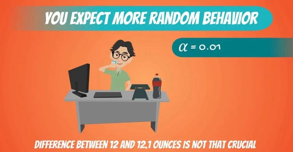
However, if we are analyzing humans or companies, we would expect more random or at least uncertain behavior. Hence, a higher degree of error.
For instance, if we want to predict how much Coca Cola its consumers drink on average, the difference between 12 ounces and 12.1 ounces will not be that crucial. So, we can choose a higher significance level like 0.05 or 0.1.
Hypothesis Testing: Performing a Z-Test
Now that we have an idea about the significance level, let’s get to the mechanics of hypothesis testing.
Imagine you are consulting a university and want to carry out an analysis on how students are performing on average.
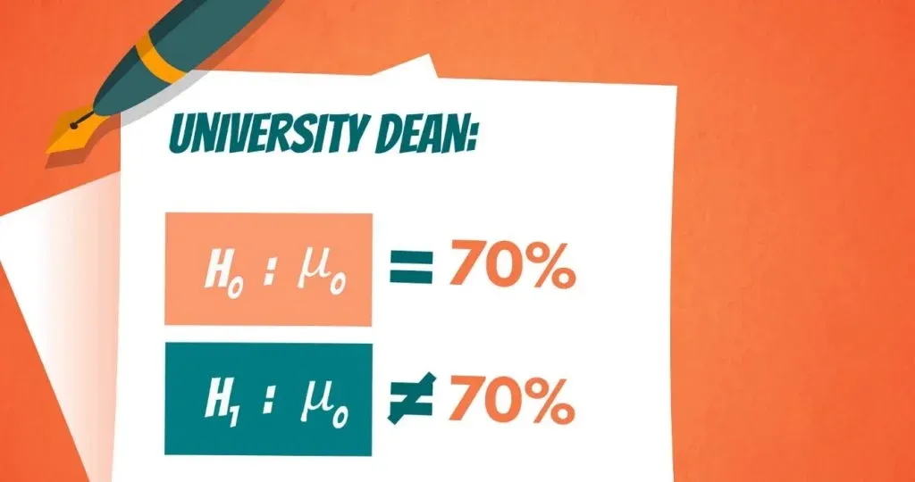
The university dean believes that on average students have a GPA of 70%. Being the data-driven researcher that you are, you can’t simply agree with his opinion, so you start testing.
The null hypothesis is: The population mean grade is 70%.
This is a hypothesized value.
The alternative hypothesis is: The population mean grade is not 70%. You can see how both of them are denoted, below.
Visualizing the Grades
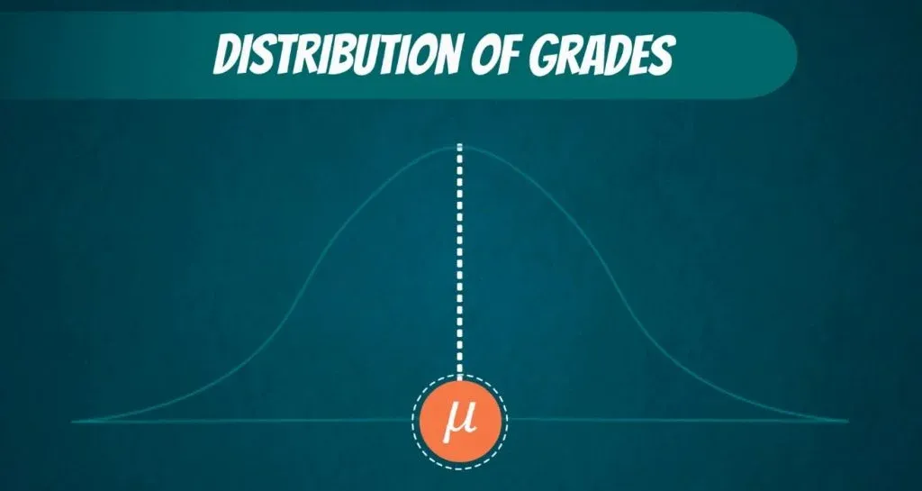
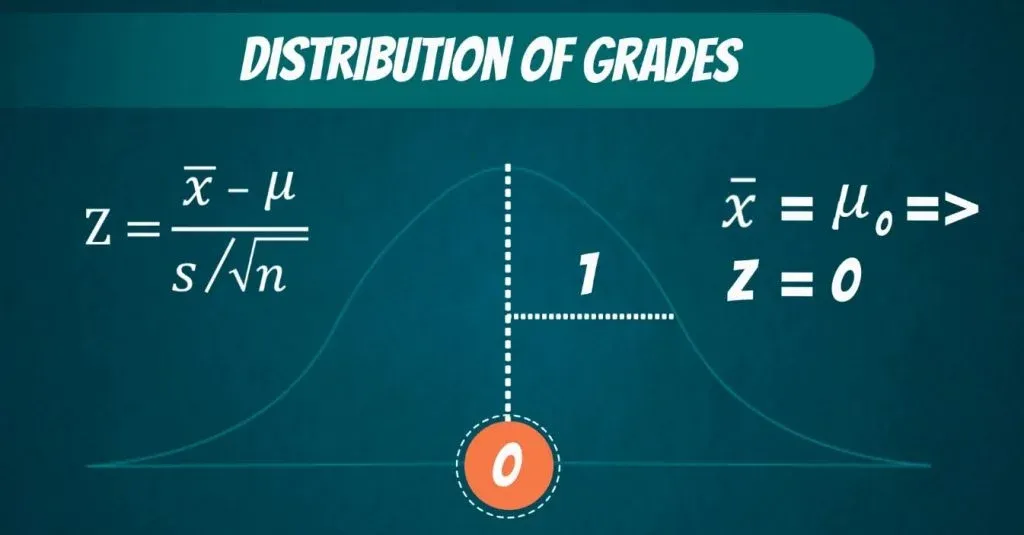
Assuming that the population of grades is normally distributed, all grades received by students should look in the following way.
That is the true population mean.
Performing a Z-test
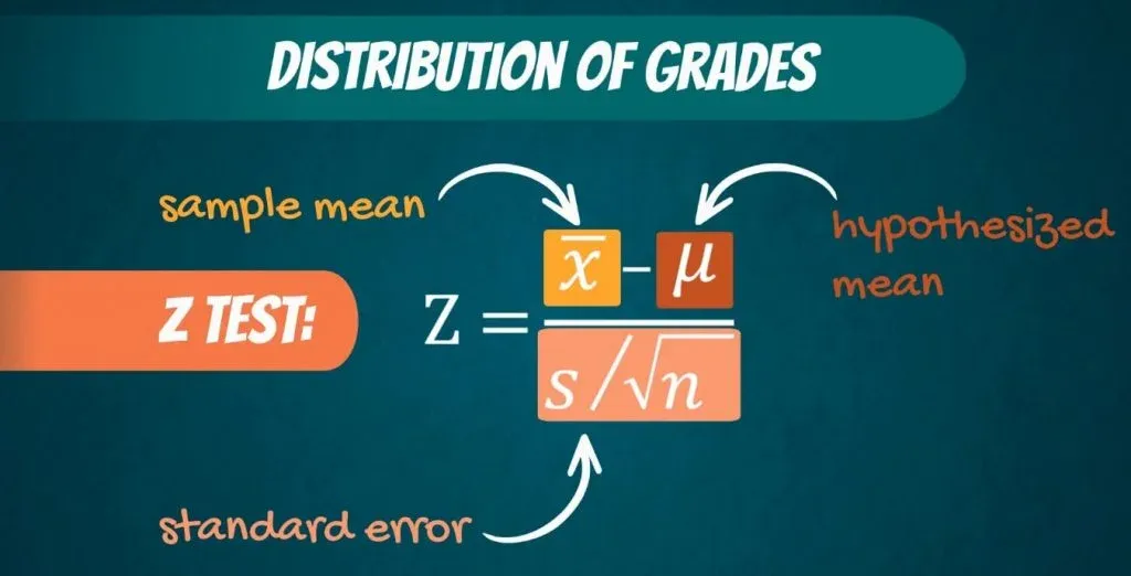
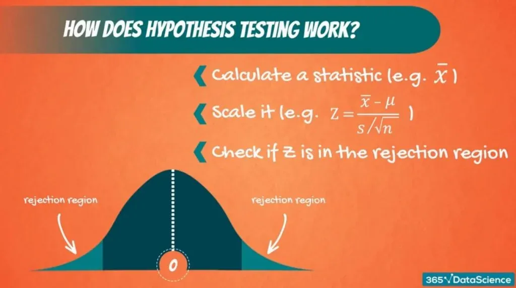
Now, a test we would normally perform is the Z-test. The formula is:
Z equals the sample mean, minus the hypothesized mean, divided by the standard error.
The idea is the following.
We are standardizing or scaling the sample mean we got. (You can quickly obtain it with our Mean, Median, Mode calculator.) If the sample mean is close enough to the hypothesized mean, then Z will be close to 0. Otherwise, it will be far away from it. Naturally, if the sample mean is exactly equal to the hypothesized mean, Z will be 0.
In all these cases, we would accept the null hypothesis.
What Is the Rejection Region?
The question here is the following:
How big should Z be for us to reject the null hypothesis?
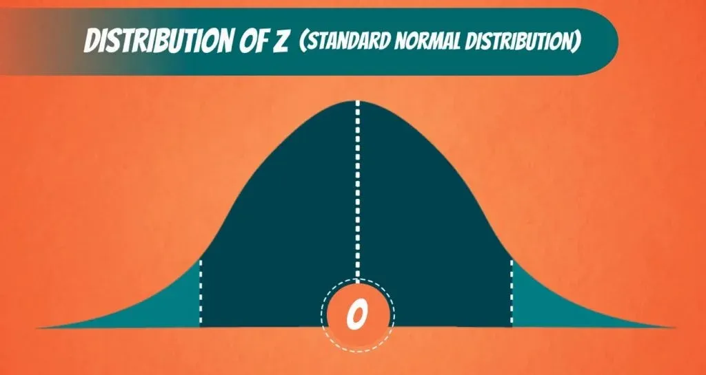
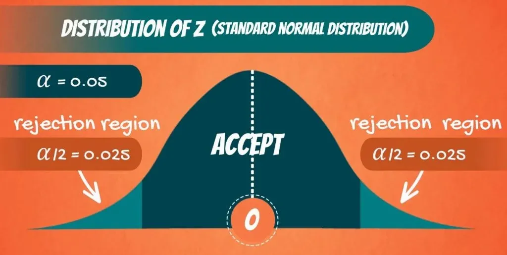
Well, there is a cut-off line. Since we are conducting a two-sided or a two-tailed test, there are two cut-off lines, one on each side.
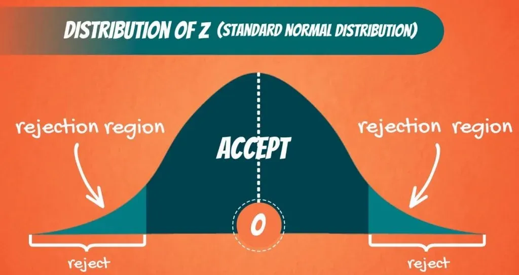
When we calculate Z, we will get a value. If this value falls into the middle part, then we cannot reject the null. If it falls outside, in the shaded region, then we reject the null hypothesis.
That is why the shaded part is called: rejection region, as you can see below.
What Does the Rejection Region Depend on?
The area that is cut-off actually depends on the significance level.
Say the level of significance, α, is 0.05. Then we have α divided by 2, or 0.025 on the left side and 0.025 on the right side.
Now these are values we can check from the z-table. When α is 0.025, Z is 1.96. So, 1.96 on the right side and minus 1.96 on the left side.
Therefore, if the value we get for Z from the test is lower than minus 1.96, or higher than 1.96, we will reject the null hypothesis. Otherwise, we will accept it.
That’s more or less how hypothesis testing works.
We scale the sample mean with respect to the hypothesized value. If Z is close to 0, then we cannot reject the null. If it is far away from 0, then we reject the null hypothesis.
Example of One Tailed Test
What about one-sided tests? We have those too!
Let’s consider the following situation.
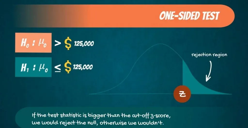
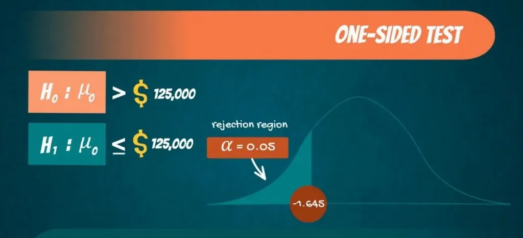
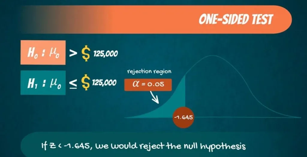
Paul says data scientists earn more than $125,000. So, H0 is: μ0 is bigger than $125,000.
The alternative is that μ0 is lower or equal to 125,000.
Using the same significance level, this time, the whole rejection region is on the left. So, the rejection region has an area of α. Looking at the z-table, that corresponds to a Z-score of 1.645. Since it is on the left, it is with a minus sign.
Accept or Reject
Now, when calculating our test statistic Z, if we get a value lower than -1.645, we would reject the null hypothesis. We do that because we have statistical evidence that the data scientist salary is less than $125,000. Otherwise, we would accept it.
Another One-Tailed Test
To exhaust all possibilities, let’s explore another one-tailed test.
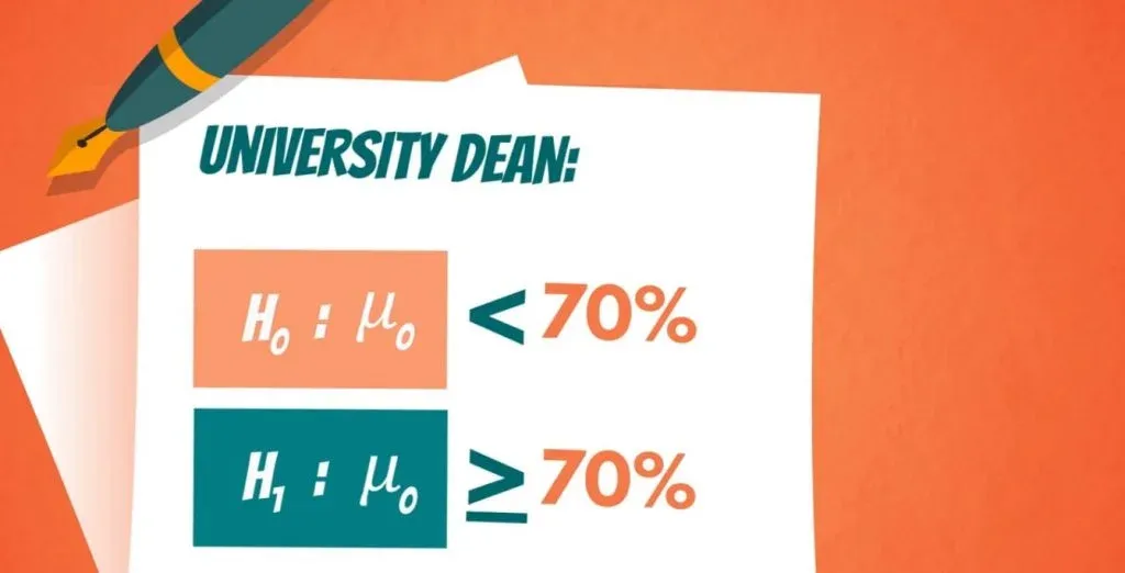
Say the university dean told you that the average GPA students get is lower than 70%. In that case, the null hypothesis is:
μ0 is lower than 70%.
While the alternative is:
μ0` is bigger or equal to 70%.
In this situation, the rejection region is on the right side. So, if the test statistic is bigger than the cut-off z-score, we would reject the null, otherwise, we wouldn’t.
Importance of the Significance Level and the Rejection Region
To sum up, the significance level and the reject region are quite crucial in the process of hypothesis testing. The level of significance conducts the accuracy of prediction. We (the researchers) choose it depending on how big of a difference a possible error could make. On the other hand, the reject region helps us decide whether or not to reject the null hypothesis. After reading this and putting both of them into use, you will realize how convenient they make your work.
***
Interested in taking your skills from good to great? Try statistics course for free!
Next Tutorial: Providing a Few Linear Regression Examples

